A key idea in data science and statistics is the Bernoulli distribution, named after the Swiss mathematician Jacob Bernoulli. It is crucial to probability theory and a building block for more complex statistical models, ranging from machine learning algorithms to predicting customer behavior. In this article, we will analyze the Bernoulli distribution in detail.
Keep reading!

What is a Bernoulli distribution?
A Bernoulli distribution is a discrete probability distribution that represents a random variable with only two possible outcomes. Typically, these results are indicated by the terms “success” and “failure” or, alternatively, by the numbers 1 and 0.
Let x be a random variable. Then, x is said to follow a Bernoulli distribution with probability of success p
The probability mass function of the Bernoulli distribution
Let x be a random variable that follows a Bernoulli distribution:

Then the probability mass function of x is

This follows directly from the definition given above.
Mean of the Bernoulli distribution
Let x be a random variable that follows a Bernoulli distribution:

Then the mean or expected value of x is
Proof: The expected value is the probability-weighted average of all possible values:

Since there are only two possible outcomes for a Bernoulli random variable, we have:

Sources: https://en.wikipedia.org/wiki/Bernoulli_distribution#Mean.
Also read: End-to-End Statistics for Data Science
Variance of the Bernoulli distribution
Let x be a random variable that follows a Bernoulli distribution:

Then the variance of x is

Proof: The variance is the probability-weighted average of the squared deviation from the expected value across all possible values.

and can also be written in terms of the expected values:
Equation (1)

The mean of a Bernoulli random variable is
Equation(2)

and the mean of a Bernoulli random variable squared is
Equation(3)

Combining equations (1), (2) and (3), we have:
Bernoulli Distribution vs Binomial Distribution
The Bernoulli distribution is a special case of the binomial distribution where the number of trials n=1. Here is a detailed comparison between the two:
| Aspect | Bernoulli Distribution | Binomial Distribution |
| Aim | Models the outcome of a single test of an event. | Models the outcome of multiple trials of the same event. |
| Representation | x∼Bernoulli(p), where p is the probability of success. | x∼Binomial(n,p), where n is the number of trials and p is the probability of success in each trial. |
| Mean | e(x)=p | e(x)=n⋅p |
| Difference | Var(x)=p(1−p) | Var(x)=n⋅p⋅(1−p) |
| Support | The results are x∈{0,1}, which represent failure (0) and success (1). | The results are x∈{0,1,2,…,n}, which represents the number of successes in n trials. |
| Special case relationship | A Bernoulli distribution is a special case of the binomial distribution when n=1. | A binomial distribution generalizes the Bernoulli distribution for n>1. |
| Example | If the probability of winning a game is 60%, the Bernoulli distribution can model whether you win (1) or lose (0) in a single game. | If the probability of winning a game is 60%, the binomial distribution can model the probability of winning exactly 3 out of 5 games. |

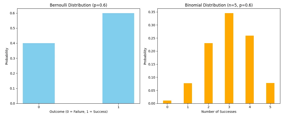
The Bernoulli distribution (left) models the outcome of a single trial with two possible outcomes: 0 (failure) or 1 (success). In this example, with p=0.6 there is a 40% chance of failure (P(x=0)=0.4) and a 60% chance of success (P(x=1)=0.6) . The graph clearly shows two bars, one for each outcome, where the height corresponds to their respective probabilities.
The binomial distribution (right) represents the number of successes across multiple trials (in this case, n=5 trials). It shows the probability of observing each possible number of successes, ranging from 0 to 5. The number of trials n and the probability of success p=0.6 influence the shape of the distribution. Here, the highest probability occurs at x=3, indicating that it is most likely to achieve exactly 3 successes in 5 attempts. The probabilities of fewer (x=0.1,2) or more (x=4.5) successes decrease symmetrically around the mean E(x)=n⋅p=3.
Also Read: A Guide to Completing Statistics for Data Science Beginners!
Using Bernoulli Distributions in Real World Applications
The Bernoulli distribution is widely used in real-world applications involving binary outcomes. Bernoulli distributions are essential for machine learning when it comes to binary classification questions. In these situations, we must classify the data into one of two groups. Examples include:
- Email spam detection (spam or non-spam)
- Fraud detection in financial transactions (legal or fraudulent)
- Diagnosis of the disease based on symptoms (absent or present)
- Medical Tests: Determine if a treatment is effective (positive/negative result).
- Games: Model the results of a single event, such as winning or losing.
- Churn analysis: predicting whether a customer will leave a service or stay.
- Sentiment analysis: Classify the text as positive or negative.
Why use the Bernoulli distribution?
- Simplicity: It is ideal for scenarios where there are only two possible outcomes.
- building block: The Bernoulli distribution serves as the basis for Binomial and other advanced distributions.
- interpretable: Real-world outcomes like success/failure, approval/rejection, or yes/no fit naturally into your framework.
Numerical example of the Bernoulli distribution:
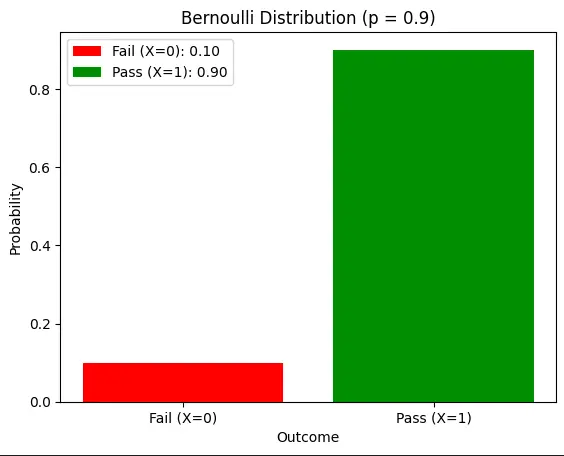
A factory produces light bulbs. Each bulb has a 90% chance of passing the quality test (p=0.9) and a 10% chance of failing (1−p=0.1). Let x be the random variable that represents the result of the quality test:
Problem:
- What is the probability that the light bulb passes the test?
- What is the expected value E(x)?
- What is the variance Var(x)?
Solution:
- Probability of passing the test: Using the Bernoulli PMF:

So the probability of passing is 0.9 (90%).
- Expected value E(x)
E(x)=p.
Here, p=0.9.
E(x)=0.9..
This means that the average success rate is 0.9 (90%).
- Variance Var(x)
Var(x)=p(1−p)
Here, p=0.9:
Var(x)=0.9(1−0.9)=0.9⋅0.1=0.09.
The variance is 0.09.
Final answer:
- Probability of passing: 0.9 (90%).
- Expected value: 0.9.
- Difference: 0.09.
This example shows how the Bernoulli distribution models single binary events as the result of a quality test.
Now let's see how this question can be solved in Python.
Implementation
Step 1 – Install the necessary library
You need to install matplotlib if you haven't already:
pip install matplotlibStep 2: Import the packages
Now, import the necessary packages for the plot and the Bernoulli distribution.
import matplotlib.pyplot as plt
from scipy.stats import bernoulli
Step 3: Define the probability of success
Set the given probability of success for the Bernoulli distribution.
p = 0.9Step 4: Calculate the PMF for success and failure
Calculate the probability mass function (PMF) for the results “Fail” (x=0) and “Pass” (x=1).
probabilities = (bernoulli.pmf(0, p), bernoulli.pmf(1, p))Step 5: Set labels for results
Define labels for the results (“Fail” and “Pass”).
outcomes = ('Fail (x=0)', 'Pass (x=1)')Step 6: Calculate the expected value
The expected value (mean) of the Bernoulli distribution is simply the probability of success.
expected_value = p # Mean of Bernoulli distributionStep 7: Calculate the variance
The variance of a Bernoulli distribution is calculated using the formula Var(x)=p(1−p)
variance = p * (1 - p) # Variance formulaStep 8: Show the results
Print the calculated probabilities, expected value, and variance.
print("Probability of Passing (x = 1):", probabilities(1))
print("Probability of Failing (x = 0):", probabilities(0))
print("Expected Value (E(x)):", expected_value)
print("Variance (Var(x)):", variance)
Production:

Step 9: Plot the probabilities
Create a bar plot for the probabilities of failure and success using matplotlib.
bars = plt.bar(outcomes, probabilities, color=('red', 'green'))Step 10: Add Title and Tags to the Plot
Set the title and labels for the x and y axes of the chart.
plt.title(f'Bernoulli Distribution (p = {p})')
plt.xlabel('Outcome')
plt.ylabel('Probability')
Step 10: Add tags to the legend
Add labels for each bar to the legend, showing the probabilities of “Fail” and “Pass.”
bars(0).set_label(f'Fail (x=0): {probabilities(0):.2f}')
bars(1).set_label(f'Pass (x=1): {probabilities(1):.2f}')
Step 11: Display the legend
Displays the legend in the plot.
plt.legend()Step 12: Show the plot
Finally, show the plot.
plt.show()
This step-by-step breakdown allows you to create the graph and calculate the values needed for the Bernoulli distribution.
Conclusion
A key idea in statistics is the Bernoulli distribution model scenarios with two possible outcomes: success or failure. It is used in many different applications, such as quality testing, consumer behavior prediction, and machine learning for binary categorization. Key characteristics of the distribution, such as variance, expected value, and probability mass function (PMF), help understand and analyze such binary events. You can create more complex models, such as the binomial distribution, if you master the Bernoulli distribution.
Frequently asked questions
Answer. No, it only handles two outcomes (success or failure). For more than two outcomes, other distributions are used, such as the multinomial distribution.
Answer. Some examples of Bernoulli trails are:
1. Flip a coin (heads or tails)
2. Pass a quality test (pass or fail)
Answer. The Bernoulli distribution is a discrete probability distribution that represents a random variable with two possible outcomes: success (1) and failure (0). It is defined by the probability of success, denoted by p.
Answer. When the number of trials (n) is equal to 1, the Bernoulli distribution is a particular case of the binomial distribution. The binomial distribution models several trials, while the Bernoulli distribution models only one.


