Understanding Overfitting in ConvNets

Introduction

Overfitting in ConvNets is a challenge in deep learning and neural networks, where a model learns too much from training data, leading to poor performance on new data. This phenomenon is especially prevalent in complex neural architectures, which can model intricate relationships. Addressing overfitting in convnet is crucial for building reliable neural network models. This article provides a guide to understanding and mitigating overfitting, examining root causes like model complexity, limited training data, and noisy features. It also discusses techniques to prevent overfitting, such as data augmentation strategies and regularization methods.

I would recommend reading these articles for basic understanding in overfitting, underfitting and bias variance tradeoff.

Learn Objectives

• Understand the causes, consequences, and scenarios of overfitting in ConvNets.
• Interpret learning curves to detect overfitting and underfitting in neural network models.
• Learn various techniques to mitigate overfitting, such as early stopping, dropout, batch normalization, regularization, and data augmentation.
• Implement these techniques using TensorFlow and Keras to train ConvNets on the CIFAR-10 dataset.
• Analyze the impact of different techniques on model performance and generalization.

Common Scenarios for Overfitting in ConvNet

Let us look into some common scenarios of overfitting in ConvNet:

Scenario1: Highly Complex Model with Insufficient Data

Using a very complex model, such as a deep neural network, on a small dataset can lead to overfitting. The model may memorize the training examples instead of learning the general pattern. For instance, training a deep neural network with only a few hundred images for a complex task like image recognition could lead to overfitting.

Consequence

The model may perform very well on the training data but fail to generalize to new, unseen data, resulting in poor performance in real-world applications.

How to resolve this issue?

Get more training data, Do image augmentation to generalize our dataset. Start with a less complex model and if the capacity is less then increase the complexity. 

Scenario2: Excessive Training

Continuously training a model for too many epochs can lead to overfitting. As the model sees the training data repeatedly, it may start to memorize it rather than learn the underlying patterns.

Consequence

The model’s performance may plateau or even degrade on unseen data as it becomes increasingly specialized to the training set.

How to resolve this issue?

Use early stopping to avoid the model to overfit and save the best model. 

Scenario3: Ignoring regularization

Regularization techniques, such as L1 or L2 regularization, are used to prevent overfitting by penalizing complex models. Ignoring or improperly tuning regularization parameters can lead to overfitting.

Consequence

The model may become overly complex and fail to generalize well to new data, resulting in poor performance outside of the training set.

How to resolve this issue?

Implement regularization, Cross-validation, Hyper parameter tuning. 

What is Model’s Capacity?

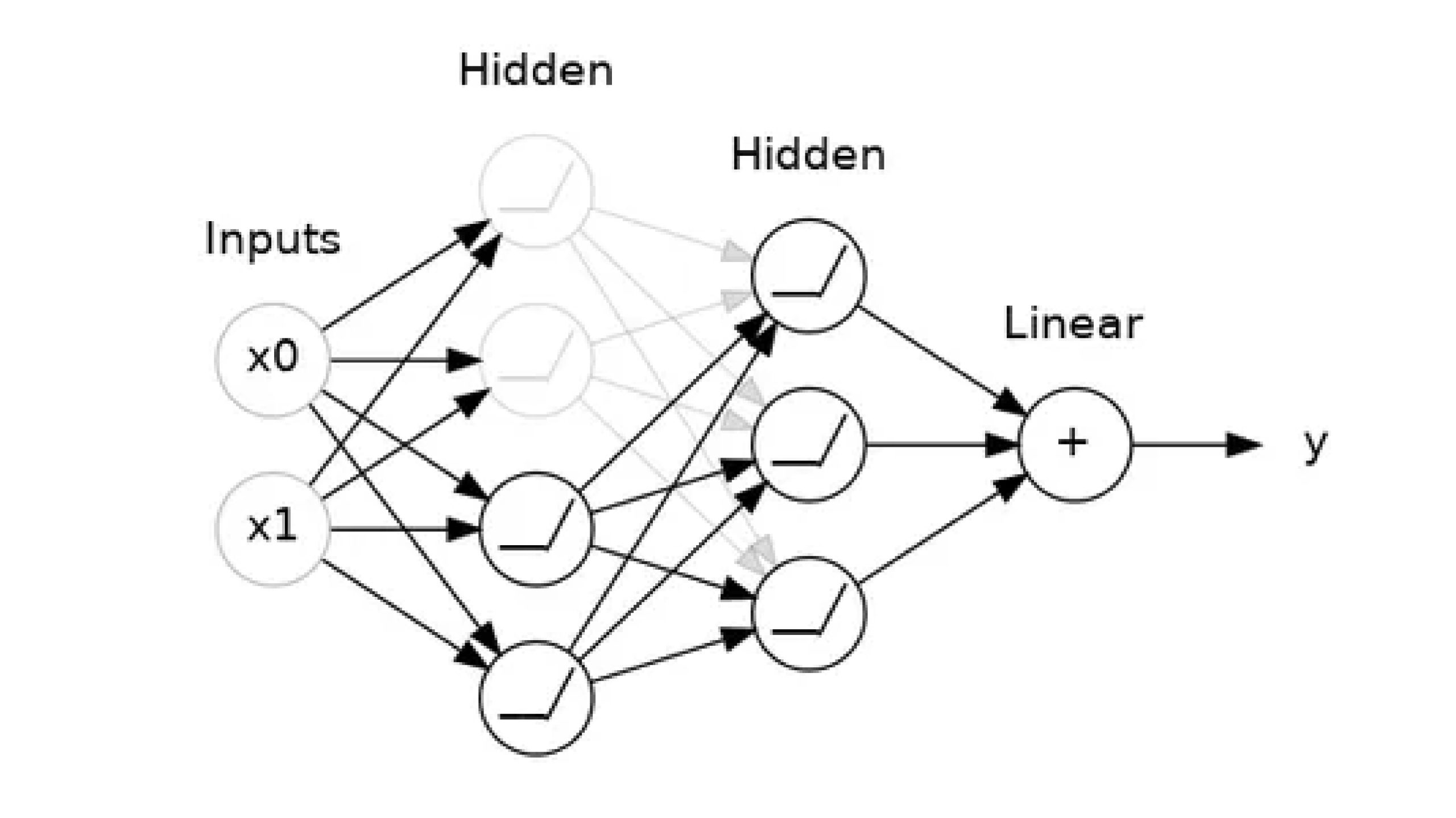
A model’s capacity refers to the size and complexity of the patterns it is able to learn. For neural networks, this will largely be determined by how many neurons it has and how they are connected together. If it appears that your network is underfitting the data, you should try increasing its capacity.

You can increase the capacity of a network either by making it wider (more units to existing layers) or by making it deeper (adding more layers). Wider networks have an easier time learning more linear relationships, while deeper networks prefer more nonlinear ones. Which is better just depends on the dataset.

Interpretation of Learning Curves

Keras provides the capability to register callbacks when training a deep learning model. One of the default callbacks registered when training all deep learning models is the History callback. It records training metrics for each epoch. This includes the loss and the accuracy (for classification problems) and the loss and accuracy for the validation dataset if one is set.

The history object is returned from calls to the fit() function used to train the model. Metrics are stored in a dictionary in the history member of the object returned.

For example, you can list the metrics collected in a history object using the following snippet of code after a model is trained:

# list all data in history
print(history.history.keys())

Output:

(‘accuracy’, ‘loss’, ‘val_accuracy’, ‘val_loss’)

Information Type

You might think about the information in the training data as being of two kinds:

• Signal: The signal is the part that generalizes, the part that can help our model make predictions from new data.
• Noise: The noise is that part that is only true of the training data; the noise is all of the random fluctuation that comes from data in the real-world or all of the incidental, non-informative patterns that can’t actually help the model make predictions. The noise is the part might look useful but really isn’t.

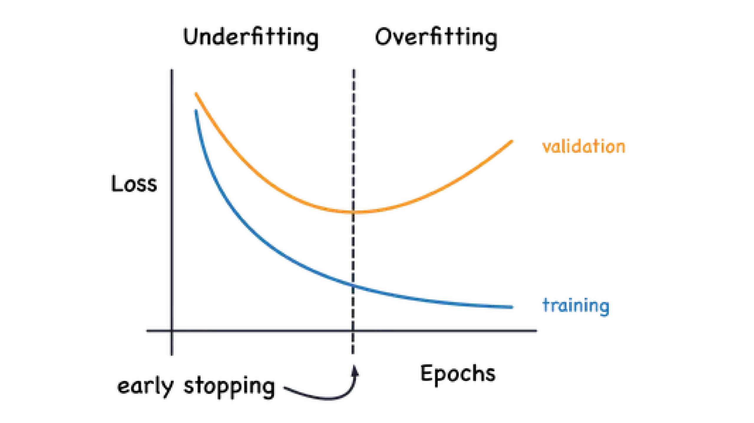
When we train a model we’ve been plotting the loss on the training set epoch by epoch. To this we’ll add a plot of the validation data too. These plots we call the learning curves. To train deep learning models effectively, we need to be able to interpret them.

In the above figure we can see that the training loss decreases as the epochs increase, but validation loss decreases at first and increases as the model starts to capture noise present in the dataset. Now we are going to see how to avoid overfitting in ConvNets through various techniques. 

Methods to Avoid Overfitting

Now that we have seen some scenarios and how to interpret learning curves to detect overfitting. let’s checkout some methods to avoid overfitting in a neural network:

Method1: Use more data

Increasing the size of your dataset can help the model generalize better as it has more diverse examples to learn from. Model will find important patterns present in the dataset and ignore noise as the model realizes those specific patterns(noise) are not present in all of the dataset.

Method2: Early Stopping

Early stopping is a technique used to prevent overfitting by monitoring the performance of the model on a validation set during training. Training is stopped when the performance on the validation set starts to degrade, indicating that the model is beginning to overfit. Typically, a separate validation set is used to monitor performance, and training is stopped when the performance has not improved for a specified number of epochs.

Method3: Dropout

We know that overfitting is caused by the network learning spurious patterns(noise) in the training data. To recognize these spurious patterns a network will often rely on very a specific combinations of weight, a kind of “conspiracy” of weights. Being so specific, they tend to be fragile: remove one and the conspiracy falls apart.

This is the idea behind dropout. To break up these conspiracies, we randomly drop out some fraction of a layer’s input units every step of training, making it much harder for the network to learn those spurious patterns in the training data. Instead, it has to search for broad, general patterns, whose weight patterns tend to be more robust. 

You could also think about dropout as creating a kind of ensemble of networks. The predictions will no longer be made by one big network, but instead by a committee of smaller networks. Individuals in the committee tend to make different kinds of mistakes, but be right at the same time, making the committee as a whole better than any individual. (If you’re familiar with random forests as an ensemble of decision trees, it’s the same idea.)

Method4: Batch Normalization

The next special method we’ll look at performs “batch normalization” (or “batchnorm”), which can help correct training that is slow or unstable.

With neural networks, it’s generally a good idea to put all of your data on a common scale, perhaps with something like scikit-learn’s StandardScaler or MinMaxScaler. The reason is that SGD will shift the network weights in proportion to how large an activation the data produces. Features that tend to produce activations of very different sizes can make for unstable training behavior.

Now, if it’s good to normalize the data before it goes into the network, maybe also normalizing inside the network would be better! In fact, we have a special kind of layer that can do this, the batch normalization layer. A batch normalization layer looks at each batch as it comes in, first normalizing the batch with its own mean and standard deviation, and then also putting the data on a new scale with two trainable rescaling parameters. Batchnorm, in effect, performs a kind of coordinated rescaling of its inputs.

Most often, batchnorm is added as an aid to the optimization process (though it can sometimes also help prediction performance). Models with batchnorm tend to need fewer epochs to complete training. Moreover, batchnorm can also fix various problems that can cause the training to get “stuck”. Consider adding batch normalization to your models, especially if you’re having trouble during training.

Method5: L1 and L2 Regularization

L1 and L2 regularization are techniques used to prevent overfitting by penalizing large weights in the neural network. L1 regularization adds a penalty term to the loss function proportional to the absolute value of the weights. It encourages sparsity in the weights and can lead to feature selection. L2 regularization, also known as weight decay, adds a penalty term proportional to the square of the weights to the loss function. It prevents the weights from becoming too large and encourages the distribution of weights to be spread out more evenly.

The choice between L1 and L2 regularization often depends on the specific problem and the desired properties of the model.

Having large values for L1/L2 regularization will cause the model not to learn fast and reach a plateau in learning causing the model to underfit. 

Method6: Data Augmentation

The best way to improve the performance of a machine learning model is to train it on more data. The more examples the model has to learn from, the better it will be able to recognize which differences in images matter and which do not. More data helps the model to generalize better.

One easy way of getting more data is to use the data you already have. If we can transform the images in our dataset in ways that preserve the class(example: MNIST Digit classification if we try augment 6 it will be difficult to distinguish between 6 and 9), we can teach our classifier to ignore those kinds of transformations. For instance, whether a car is facing left or right in a photo doesn’t change the fact that it is a Car and not a Truck. So, if we augment our training data with flipped images, our classifier will learn that “left or right” is a difference it should ignore.

And that’s the whole idea behind data augmentation: add in some extra fake data that looks reasonably like the real data and your classifier will improve. 

Remember, the key to avoiding overfitting is to make sure your model generalizes well. Always check your model’s performance on a validation set, not just the training set.

Implementation of Above Methods with Data

Let us explore implementation steps for above methods:

Step1: Loading Necessary Libraries

import numpy as np
import pandas as pd
import matplotlib.pyplot as plt
import tensorflow as tf
from tensorflow.keras import datasets, layers, models
from tensorflow.keras.preprocessing.image import ImageDataGenerator
from tensorflow.keras.callbacks import ModelCheckpoint
import keras
from keras.preprocessing import image
from keras import models, layers, regularizers
from tqdm import tqdm
import warnings
warnings.filterwarnings(action='ignore')

Step2: Loading Dataset and Preprocessing

#Here all the images are in the form of a numpy array
cifar10 = tf.keras.datasets.cifar10
(x_train, y_train), (x_test, y_test) = cifar10.load_data()
x_train = x_train / 255.0
x_test = x_test / 255.0

Step3: Learning Dataset

x_train.shape, y_train.shape, x_test.shape, y_test.shape 

Output:

np.unique(y_train)

Output:

#These labels are in the order and taken from the documentaion
class_names = ('airplane', 'automobile', 'bird', 'cat', 'deer',
               'dog', 'frog', 'horse', 'ship', 'truck')

Step4: Visualizing image From Dataset

def show_image(IMG_INDEX):
    plt.imshow(x_train(20) ,cmap=plt.cm.binary)
    plt.xlabel(class_names(y_train(IMG_INDEX)(0)))
    plt.show()
show_image(20)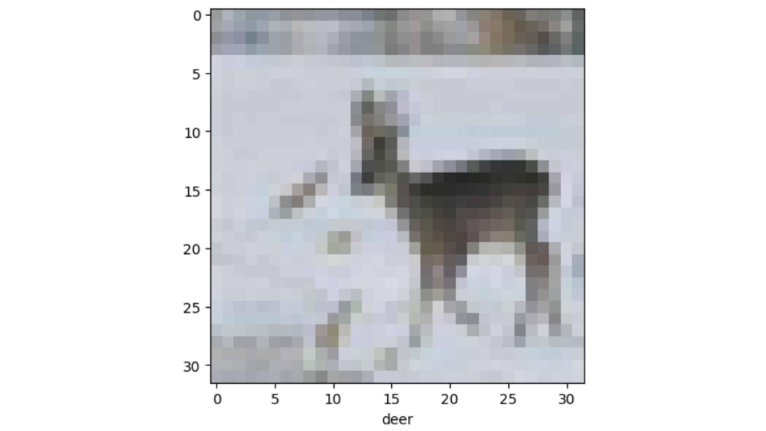

model = models.Sequential()
model.add(layers.Conv2D(32, (3, 3), activation='relu', input_shape=(32, 32, 3)))
model.add(layers.AveragePooling2D((2, 2)))
model.add(layers.Conv2D(64, (3, 3), activation='relu'))
model.add(layers.AveragePooling2D((2, 2)))
model.add(layers.Conv2D(64, (3, 3), activation='relu'))
model.add(layers.Flatten())
model.add(layers.Dense(64, activation='relu'))
model.add(layers.Dense(10))
model.summary()

Let us now Initialize hyper parameters and compiling model with optimizer, loss function and evaluation metric.

train_hyperparameters_config={'optim':keras.optimizers.Adam(learning_rate=0.001),
                             'epochs':20,
                              'batch_size':16
                             }
model.compile(optimizer=train_hyperparameters_config('optim'),
                  loss=tf.keras.losses.SparseCategoricalCrossentropy(from_logits=True),
                  metrics=('accuracy'))

Step6: Training Model

history = model.fit(x_train, y_train, 
                        epochs=train_hyperparameters_config('epochs'), 
                        batch_size=train_hyperparameters_config('batch_size'), 
                        verbose=1,
                        validation_data=(x_test, y_test))

Step7: Evaluate the Model

These will tell us the information contained in history object and we use those to create our information curves.

print(history.history.keys()) 

def learning_curves(history):
# Plotting Accuracy
    plt.figure(figsize=(14, 5))  # Adjust the figure size as needed
    plt.subplot(1, 2, 1)  # Subplot with 1 row, 2 columns, and index 1
    plt.plot(history.history('accuracy'), label="train_accuracy", marker="s", markersize=4)
    plt.plot(history.history('val_accuracy'), label="val_accuracy", marker="*", markersize=4)
    plt.xlabel('Epoch')
    plt.ylabel('Accuracy')
    plt.legend(loc="lower right")

    # Plotting Loss
    plt.subplot(1, 2, 2)  # Subplot with 1 row, 2 columns, and index 2
    plt.plot(history.history('loss'), label="train_loss", marker="s", markersize=4)
    plt.plot(history.history('val_loss'), label="val_loss", marker="*", markersize=4)
    plt.xlabel('Epoch')
    plt.ylabel('Loss')
    plt.legend(loc="lower right")

    plt.show()
learning_curves(history)

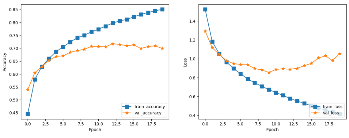
From the curves we can see that the validation accuracy reaches a plateau after the 4th epoch and the model starts to capture noise. Hence we will implement early stopping to avoid model from overfitting and restore the best weights based on val_loss. We will use val_loss to monitor early stopping as our neural network tries to reduce loss using optimizers. Accuracy and Validation accuracy depend on the threshold(A probability to separate classes – usually 0.5 for binary classification), so if our dataset is imbalanced it would be loss we should worry about in most of the cases. 

Step8: Implementing Early Stopping

Since we are not worried about our model to overfit as early stopping will avoid our model from happening. It is a good choice to choose a higher number of epochs and a suitable patience. Now we will use the same model architecture and train with early stopping callback. 

model = models.Sequential()
model.add(layers.Conv2D(32, (3, 3), activation='relu', input_shape=(32, 32, 3)))
model.add(layers.AveragePooling2D((2, 2)))
model.add(layers.Conv2D(64, (3, 3), activation='relu'))
model.add(layers.AveragePooling2D((2, 2)))
model.add(layers.Conv2D(64, (3, 3), activation='relu'))
model.add(layers.Flatten())
model.add(layers.Dense(128, activation='relu'))
model.add(layers.Dense(64, activation='relu'))
model.add(layers.Dense(10))
model.summary()

# Here we have used more epochs than needed since we use patience parameter which we stop the model from overfitting
train_hyperparameters_config = {
    'optim': keras.optimizers.Adam(learning_rate=0.001),
    'patience': 5,
    'epochs': 50,
    'batch_size': 32, 
}
print('Setting the callback and early stopping configurations...')
callback = tf.keras.callbacks.EarlyStopping(
    monitor="val_loss", 
    min_delta=0.001, # minimium amount of change to count as an improvement
    patience=train_hyperparameters_config('patience'), 
    restore_best_weights=True)

def model_train(model, x_train, y_train, x_test, y_test, train_hyperparameters_config):
    model.compile(optimizer=train_hyperparameters_config('optim'),
                      loss=tf.keras.losses.SparseCategoricalCrossentropy(from_logits=True),
                      metrics=('accuracy'))
    ht = model.fit(x_train, y_train, 
                            epochs=train_hyperparameters_config('epochs'), 
                            batch_size=train_hyperparameters_config('batch_size'),
                            callbacks=(callback),
                            verbose=1,
                            validation_data=(x_test, y_test))
    return ht

ht=model_train(model, x_train, y_train, x_test, y_test, train_hyperparameters_config)

learning_curves(ht)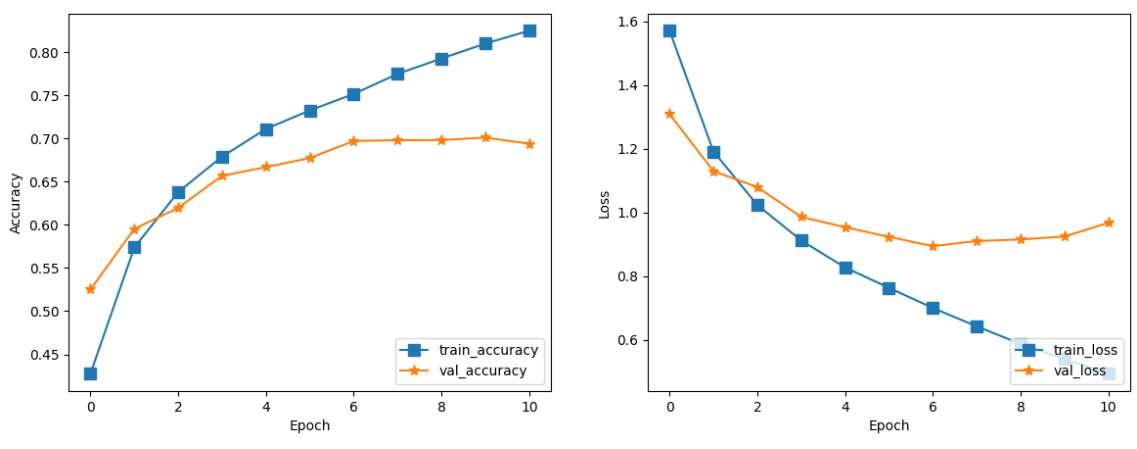

To know our best weights that the model has taken. 

print('Testing ..................')
test_loss, test_acc = model.evaluate(x_test,  y_test, verbose=2)
print('test_loss : ', test_loss, 'test_accuracy : ', test_acc)

Step9: Increasing Model Complexity

Since our model is not performing well and underfits as it is not able to capture enough data. We should increase our model complexity and evaluate. 

model = models.Sequential()

model.add(layers.Conv2D(128, (3, 3), activation='relu', input_shape=(32, 32, 3)))
model.add(layers.MaxPooling2D((2, 2)))

model.add(layers.Conv2D(256, (3, 3), activation='relu'))
model.add(layers.MaxPooling2D((2, 2)))

model.add(layers.Conv2D(256, (3, 3), activation='relu'))
model.add(layers.MaxPooling2D((2, 2)))

model.add(layers.Conv2D(512, (3, 3), activation='relu', padding='same'))
model.add(layers.MaxPooling2D((2, 2)))

model.add(layers.Flatten())
model.add(layers.Dense(256, activation='relu'))
model.add(layers.Dense(128, activation='relu'))
model.add(layers.Dense(10, activation='softmax'))
model.summary()

We can see there is an increase in the total parameters. This would help in finding more complex relationships in our model. Note: Our dataset is of 32X32 images; these are relatively small images. Hence using more complex models at the beginning will surely overfit the model hence we tend to increase our model complexity slowly.

# Here we have used more epochs than needed since we use patience parameter which we stop the model from overfitting
train_hyperparameters_config = {
    'optim': keras.optimizers.Adam(learning_rate=0.001),
    'patience': 5,
    'epochs': 50,
    'batch_size': 32, 
}
print('Setting the callback and early stopping configurations...')
callback = tf.keras.callbacks.EarlyStopping(
    monitor="val_loss", 
    min_delta=0.001, # minimium amount of change to count as an improvement
    patience=train_hyperparameters_config('patience'), 
    restore_best_weights=True)
ht=model_train(model, x_train, y_train, x_test, y_test, train_hyperparameters_config)

learning_curves(ht)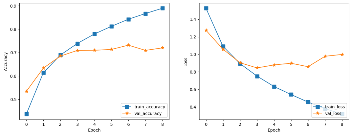

print('Testing ..................')
test_loss, test_acc = model.evaluate(x_test,  y_test, verbose=2)
print('test_loss : ', test_loss, 'test_accuracy : ', test_acc)

From the above graphs we can clearly say that the model is overfitting, hence we will use another method called Drop out normalization and Batch normalization.

Step10: Using Dropout Layers and Batch Normalization Layers

model = models.Sequential()

model.add(layers.Conv2D(128, (3, 3), activation='relu', input_shape=(32, 32, 3)))
model.add(layers.BatchNormalization())
model.add(layers.MaxPooling2D((2, 2)))

model.add(layers.Conv2D(256, (3, 3), activation='relu'))
model.add(layers.BatchNormalization())
model.add(layers.MaxPooling2D((2, 2)))

model.add(layers.Conv2D(256, (3, 3), activation='relu'))
model.add(layers.BatchNormalization())
model.add(layers.MaxPooling2D((2, 2)))

model.add(layers.Conv2D(512, (3, 3), activation='relu', padding='same'))
model.add(layers.BatchNormalization())
model.add(layers.MaxPooling2D((2, 2)))

model.add(layers.Flatten())
model.add(layers.Dense(256, activation='relu'))
model.add(layers.BatchNormalization())
model.add(layers.Dropout(0.3))

model.add(layers.Dense(128, activation='relu'))
model.add(layers.BatchNormalization())
model.add(layers.Dropout(0.3))

model.add(layers.Dense(10, activation='softmax'))
model.summary()

# Here we have used more epochs than needed since we use patience parameter which we stop the model from overfitting
train_hyperparameters_config = {
    'optim': keras.optimizers.Adam(learning_rate=0.001),
    'patience': 5,
    'epochs': 50,
    'batch_size': 32, 
}
print('Setting the callback and early stopping configurations...')
callback = tf.keras.callbacks.EarlyStopping(
    monitor="val_loss", 
    min_delta=0.001, # minimium amount of change to count as an improvement
    patience=train_hyperparameters_config('patience'), 
    restore_best_weights=True)
ht=model_train(model, x_train, y_train, x_test, y_test, train_hyperparameters_config)

learning_curves(ht)

print('Testing ..................')
test_loss, test_acc = model.evaluate(x_test,  y_test, verbose=2)
print('test_loss : ', test_loss, 'test_accuracy : ', test_acc)

From the learning graphs we can see that the model is overfitting even with batchnormalization and dropout layers. Hence instead of increasing the complexity but increasing the number of filters. We would add more convolution layers to extract more features.

Step11: Increasing Convolution Layers

Decrease the trainable parameter but increase the convolution layers to extract more features.

model = models.Sequential()

model.add(layers.Conv2D(32, (3, 3), activation='relu', padding='same', input_shape=(32, 32, 3)))
model.add(layers.BatchNormalization())
model.add(layers.Conv2D(32, (3, 3), activation='relu', padding='same'))
model.add(layers.BatchNormalization())
model.add(layers.MaxPool2D((2, 2)))
model.add(layers.Dropout(0.2))

model.add(layers.Conv2D(64, (3, 3), activation='relu', padding='same'))
model.add(layers.BatchNormalization())
model.add(layers.Conv2D(64, (3, 3), activation='relu', padding='same'))
model.add(layers.BatchNormalization())
model.add(layers.MaxPool2D((2, 2)))
model.add(layers.Dropout(0.3))

model.add(layers.Conv2D(128, (3, 3), activation='relu', padding='same'))
model.add(layers.BatchNormalization())
model.add(layers.Conv2D(128, (3, 3), activation='relu', padding='same'))
model.add(layers.BatchNormalization())
model.add(layers.MaxPool2D((2, 2)))
model.add(layers.Dropout(0.4))

model.add(layers.Flatten())
model.add(layers.Dense(128, activation='relu'))
model.add(layers.BatchNormalization())
model.add(layers.Dropout(0.5))

model.add(layers.Dense(10, activation='softmax'))

model.summary()

# Here we have used more epochs than needed since we use patience parameter which we stop the model from overfitting
train_hyperparameters_config = {
    'optim': keras.optimizers.Adam(learning_rate=0.001),
    'patience': 5,
    'epochs': 50,
    'batch_size': 32, 
}
print('Setting the callback and early stopping configurations...')
callback = tf.keras.callbacks.EarlyStopping(
    monitor="val_loss", 
    min_delta=0.001, # minimium amount of change to count as an improvement
    patience=train_hyperparameters_config('patience'), 
    restore_best_weights=True)
ht=model_train(model, x_train, y_train, x_test, y_test, train_hyperparameters_config)

learning_curves(ht)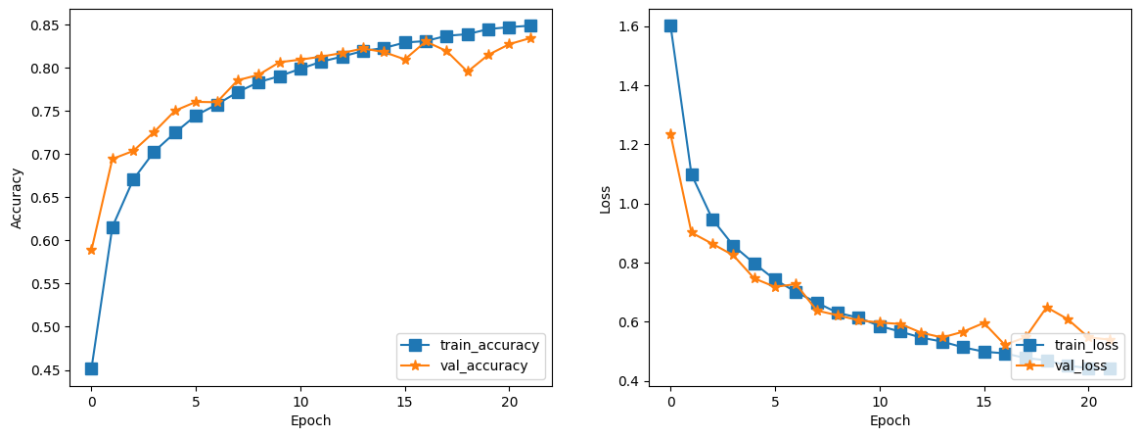

print('Testing ..................')
test_loss, test_acc = model.evaluate(x_test,  y_test, verbose=2)
print('test_loss : ', test_loss, 'test_accuracy : ', test_acc)

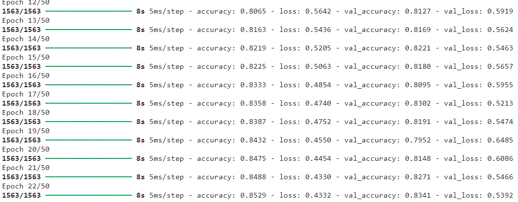
From the above output and learning curve we can infer that the model has performed very well and has avoided overfitting. The training accuracy and validation accuracy are very near. In this scenario we will not need more methods to decrease overfitting. Yet we will explore L1/L2 regularization. 

Step12: Using L1/L2 Regularization

from tensorflow.keras import regularizers

model = models.Sequential()

model.add(layers.Conv2D(32, (3, 3), activation='relu', padding='same', input_shape=(32, 32, 3)))
model.add(layers.BatchNormalization())
model.add(layers.Conv2D(32, (3, 3), activation='relu', padding='same', kernel_regularizer=regularizers.l1(0.0005)))
model.add(layers.BatchNormalization())
model.add(layers.MaxPool2D((2, 2)))
model.add(layers.Dropout(0.2))

model.add(layers.Conv2D(64, (3, 3), activation='relu', padding='same'))
model.add(layers.BatchNormalization())
model.add(layers.Conv2D(64, (3, 3), activation='relu', padding='same', kernel_regularizer=regularizers.l2(0.0005)))
model.add(layers.BatchNormalization())
model.add(layers.MaxPool2D((2, 2)))
model.add(layers.Dropout(0.3))

model.add(layers.Conv2D(128, (3, 3), activation='relu', padding='same'))
model.add(layers.BatchNormalization())
model.add(layers.Conv2D(128, (3, 3), activation='relu', padding='same'))
model.add(layers.BatchNormalization())
model.add(layers.MaxPool2D((2, 2)))
model.add(layers.Dropout(0.4))

model.add(layers.Flatten())
model.add(layers.Dense(128, activation='relu', kernel_regularizer=regularizers.l1_l2(0.0005, 0.0005)))
model.add(layers.BatchNormalization())
model.add(layers.Dropout(0.5))
model.add(layers.Dense(10, activation='softmax'))

model.summary()

# Here we have used more epochs than needed since we use patience parameter which we stop the model from overfitting
train_hyperparameters_config = {
    'optim': keras.optimizers.Adam(learning_rate=0.001),
    'patience': 7,
    'epochs': 70,
    'batch_size': 32, 
}
print('Setting the callback and early stopping configurations...')
callback = tf.keras.callbacks.EarlyStopping(
    monitor="val_loss", 
    min_delta=0.001, # minimium amount of change to count as an improvement
    patience=train_hyperparameters_config('patience'), 
    restore_best_weights=True)
ht=model_train(model, x_train, y_train, x_test, y_test, train_hyperparameters_config)

learning_curves(ht)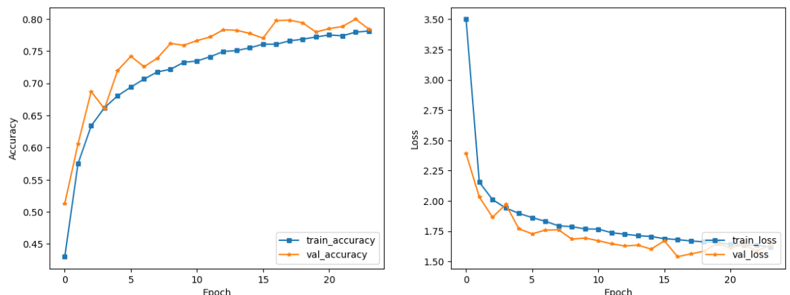

print('Testing ..................')
test_loss, test_acc = model.evaluate(x_test,  y_test, verbose=2)
print('test_loss : ', test_loss, 'test_accuracy : ', test_acc)

Now we can see that L1/L2 regularization even after using a low penalty score of 0.0001, made our model underfit by 4%. Hence it is advisable to cautiously use all the methods together. As Batch Normalization and Regularization affect the model in a similar way we would not need L1/L2 regularization. 

Step13: Data Augmentation

We will be using ImageDataGenerator from tensorflow keras.

# creates a data generator object that transforms images
datagen = ImageDataGenerator(
rotation_range=40,
width_shift_range=0.2,
height_shift_range=0.2,
shear_range=0.2,
zoom_range=0.2,
horizontal_flip=True,
fill_mode="nearest")

# pick an image to transform
test_img = x_train(20)
img = image.img_to_array(test_img)  # convert image to numpy arry
img = img.reshape((1,) + img.shape)  # reshape image

i = 0

for batch in datagen.flow(img, save_prefix='test', save_format="jpeg"):  # this loops runs forever until we break, saving images to current directory with specified prefix
    plt.figure(i)
    plot = plt.imshow(image.img_to_array(batch(0)))
    i += 1
    if i > 4:  # show 4 images
        break

plt.show()

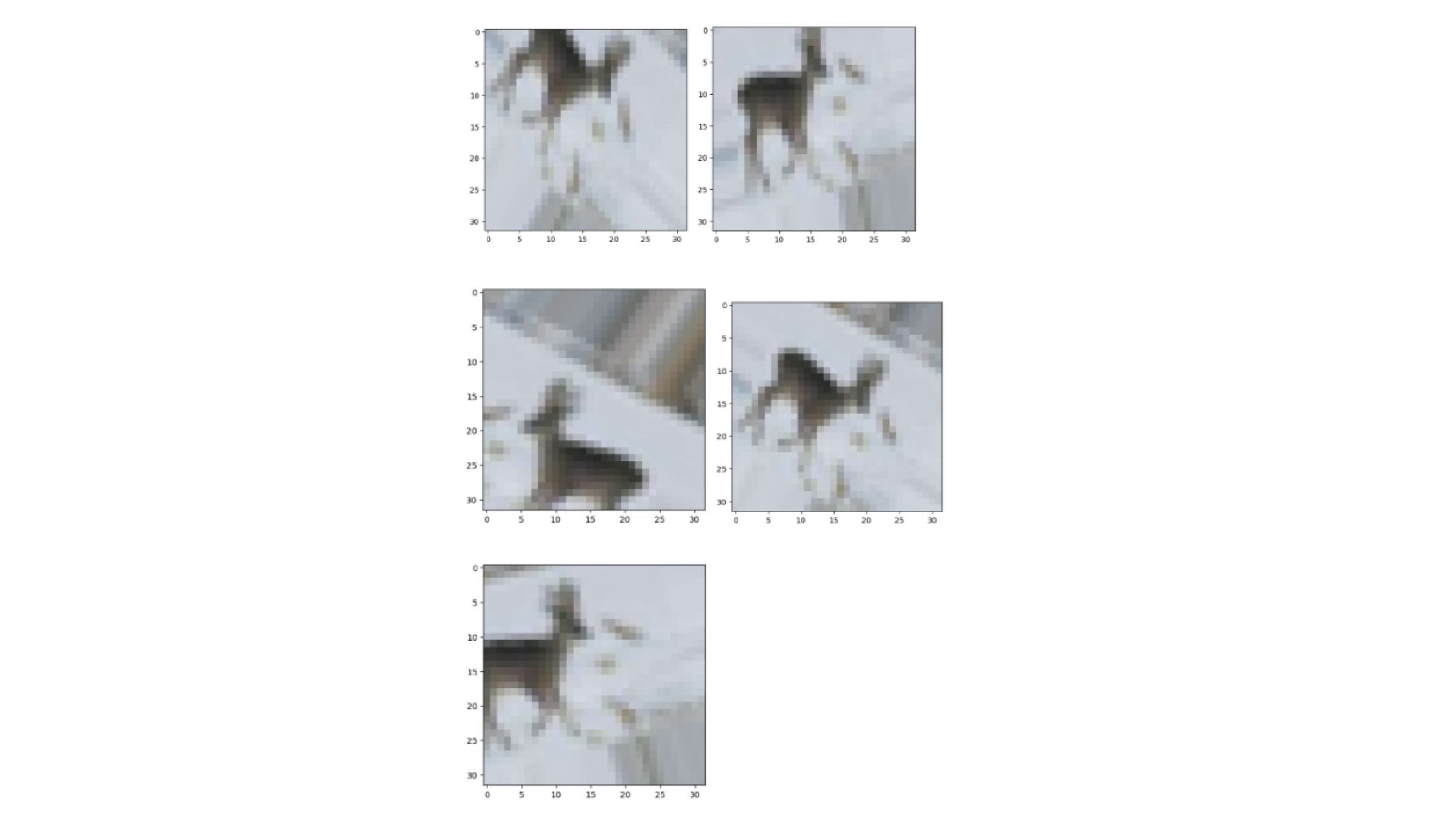
These are four augmented images and one original image.

# Create an instance of the ImageDataGenerator
datagen = ImageDataGenerator(
    rotation_range=40,
    width_shift_range=0.2,
    height_shift_range=0.2,
    shear_range=0.2,
    zoom_range=0.2,
    horizontal_flip=True,
    fill_mode="nearest"
)

# Create an iterator for the data generator
data_generator = datagen.flow(x_train, y_train, batch_size=32)

# Create empty lists to store the augmented images and labels
augmented_images = ()
augmented_labels = ()

# Loop over the data generator and append the augmented data to the lists
num_batches = len(x_train) // 32
progress_bar = tqdm(total=num_batches, desc="Augmenting data", unit="batch")

for i in range(num_batches):
    batch_images, batch_labels = next(data_generator)
    augmented_images.append(batch_images)
    augmented_labels.append(batch_labels)
    progress_bar.update(1)

progress_bar.close()

# Convert the lists to NumPy arrays
augmented_images = np.concatenate(augmented_images, axis=0)
augmented_labels = np.concatenate(augmented_labels, axis=0)

# Combine the original and augmented data
x_train_augmented = np.concatenate((x_train, augmented_images), axis=0)
y_train_augmented = np.concatenate((y_train, augmented_labels), axis=0)

We have used tqdm library to know the progress of our augmentation.

x_train_augmented.shape, y_train_augmented.shape

This is our dataset after augmentation. Now lets use this dataset and train our model.

model = models.Sequential()

model.add(layers.Conv2D(32, (3, 3), activation='relu', padding='same', input_shape=(32, 32, 3)))
model.add(layers.BatchNormalization())
model.add(layers.Conv2D(32, (3, 3), activation='relu', padding='same'))
model.add(layers.BatchNormalization())
model.add(layers.MaxPool2D((2, 2)))
model.add(layers.Dropout(0.2))

model.add(layers.Conv2D(64, (3, 3), activation='relu', padding='same'))
model.add(layers.BatchNormalization())
model.add(layers.Conv2D(64, (3, 3), activation='relu', padding='same'))
model.add(layers.BatchNormalization())
model.add(layers.MaxPool2D((2, 2)))
model.add(layers.Dropout(0.3))

model.add(layers.Conv2D(128, (3, 3), activation='relu', padding='same'))
model.add(layers.BatchNormalization())
model.add(layers.Conv2D(128, (3, 3), activation='relu', padding='same'))
model.add(layers.BatchNormalization())
model.add(layers.MaxPool2D((2, 2)))
model.add(layers.Dropout(0.4))

model.add(layers.Flatten())
model.add(layers.Dense(128, activation='relu'))
model.add(layers.BatchNormalization())
model.add(layers.Dropout(0.5))

model.add(layers.Dense(10, activation='softmax'))

model.summary()

# Here we have used more epochs than needed since we use patience parameter which we stop the model from overfitting
train_hyperparameters_config = {
    'optim': keras.optimizers.Adam(learning_rate=0.001),
    'patience': 10,
    'epochs': 70,
    'batch_size': 32, 
}
print('Setting the callback and early stopping configurations...')
callback = tf.keras.callbacks.EarlyStopping(
    monitor="val_loss", 
    min_delta=0.001, # minimium amount of change to count as an improvement
    patience=train_hyperparameters_config('patience'), 
    restore_best_weights=True)

ht=model_train(model, x_train_augmented, y_train_augmented, x_test, y_test, train_hyperparameters_config)

learning_curves(ht)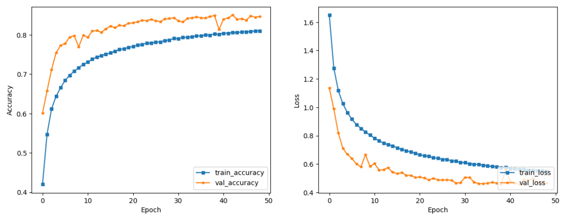

print('Testing ..................')
test_loss, test_acc = model.evaluate(x_test,  y_test, verbose=2)
print('test_loss : ', test_loss, 'test_accuracy : ', test_acc)

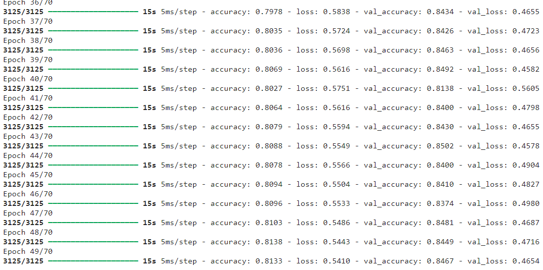
We can see the model is more generalized and a decrease in loss. We have got better validation accuracy as well. Hence data augmentation has increased our model accuracy. 

Conclusion

Overfitting is a common issue in deep learning, especially with complex neural network architectures like ConvNets. Practitioners can prevent overfitting in ConvNets by understanding its root causes and recognizing scenarios where it occurs. Techniques like early stopping, dropout, batch normalization, regularization, and data augmentation can help mitigate this issue. Implementing these techniques on the CIFAR-10 dataset showed significant improvements in model generalization and performance. Mastering these techniques and understanding their principles can lead to robust and reliable neural network models.

Frequently Asked Questions