NEWSLETTER
Introduction
The basic time series model, or TimesFM for short, is a pre-trained basic time series model developed by Google Research for forecasting univariate time series. As a pre-trained basic model, it simplifies the often complex process of time series analysis. Google Research says its basic time series model exhibits zero-shot forecasting capabilities that rival the accuracy of leading forecasting models monitored on multiple public data sets.

Overview
- TimesFM is a pretrained model developed by Google Research for univariate time series forecasting, providing zero prediction capabilities that rival leading supervised models.
- TimesFM is a transformer-based model with 200 million parameters, designed to predict future values of a single variable based on its historical data, and supports context lengths of up to 512 points.
- It displays high forecast accuracy on unseen data sets, leveraging its transformer layers and tunable hyperparameters such as model dimensions, patch lengths, and horizon lengths.
- The demo uses TimesFM on Kaggle's electricity production dataset. It shows accurate forecasts with minimal errors (e.g. MAE = 3.34) and performs well compared to actual data.
- TimesFM is an advanced model that simplifies time series analysis while achieving near-state-of-the-art accuracy in predicting future trends across multiple data sets without the need for additional training.
Background
A time series consists of data points collected at consistent time intervals, such as daily stock prices or hourly temperature readings. Forecasting such data is often complex due to elements such as trends, seasonal variations and erratic patterns. These challenges can make accurate predictions of future values difficult, but models like FM Schedules They are designed to speed up this task.
Understanding the architecture of TimesFM
TimesFM 1.0 contains a 200M parameter, decoder trained with a transformer-based model solely on a pre-training dataset with over 100 billion real-world time points.
TimesFM 1.0 generates accurate forecasts on unseen data sets without additional training; predicts future values of a single variable based on its own historical data. It involves using a variable (time series) to forecast future points of that same variable with respect to time. It performs univariate time series forecasts for context lengths up to 512 time points and, at any horizon length, has an optional frequency indicator input.
Also Read: Time Series Forecasting – Complete Tutorial | Part 1
Parameters (hyperparameters)
These are adjustable values that control the behavior of the model and impact its performance:
- dim_model: Dimensionality of the input and output vectors.
- input_patch_len (p): Length of each input patch.
- output_patch_len (h): Length of the forecast generated at each step.
- number_heads: Number of attention heads in the multi-head attention mechanism.
- num_layers (nl): Number of stacked transformer layers.
- context length (L): The length of the historical data used for prediction.
- horizon length (H): The length of the forecast horizon.
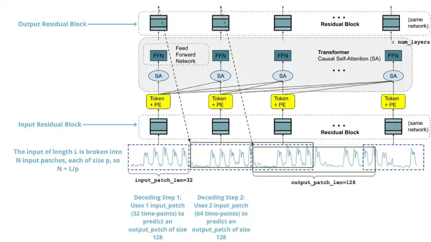
- Number of input tokens (N)calculated as the total length of the context divided by the length of the input patch: N = L/p. Each of these tokens is fed into the transformer layers for processing.
Components
These are the fundamental components of the model architecture:
- Residual blocks: Neural network blocks used to process input and output patches.
- stacked transformer: The core layers of the transformer in the model.
- tj: The input tokens fed to the transformer layers, derived from the processed patches.
t_j = InputResidualBlock(ŷ_j ⊙ (1 – m_j)) + PE_j
where ỹ_j is the jth patch of the input series, m̃_j is the corresponding mask and PE_j is the positional encoding.
- DO: He exit tab in step j, generated by the transformer layers based on the input tokens. It is used to predict the corresponding output patch:
o_j = Stacked Transformer((t_1, ṁ_1),…, (t_j, ṁ_j))
- m1:L (mask): The mask used to ignore certain parts of the input during processing.
He loss function It is used during training. In the case of the point forecast, it is the Mean square error (MSE):
Train loss = (1 / N) * Σ (MSE(ŷp(j+1):p(j+h), yp(j+1):p(j+h)))
Where ŷ are the model predictions and y are the true future values.
Also Read: Introduction to Time Series Data Forecasting
TimesFM 1.0 for forecasts
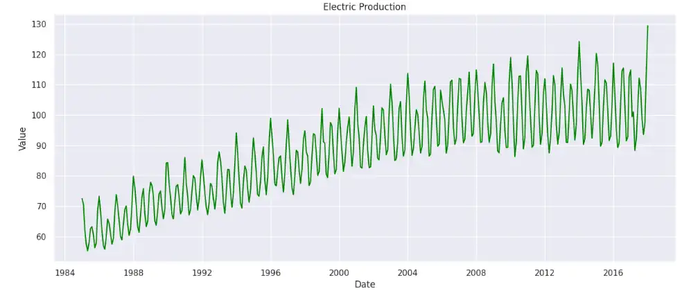
He “Electric Production” data set is available on Kaggle and contains data related to electricity production over time. It consists of only two columns: DATEwhich represents the date of the recorded securities, and Worthwhich indicates the amount of electricity produced in that month. Our task is to forecast 24 months of data using TimesFM.
Manifestation
Before you begin, make sure you are using a GPU. I am doing this demo on kaggle and will be using T4 x 2 GPU accelerator.
Let's install “timesfm” using pip, “-q” will just install it without displaying anything.
!pip -q install timesfmLet's import some necessary libraries and read the data set.
import timesfmimport pandas as pd
data=pd.read_csv('/kaggle/input/electric-production/Electric_Production.csv')
data.head()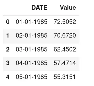
Performs univariate time series forecasts for context lengths up to 512 time points and at any horizon length, has an optional frequency indicator input.
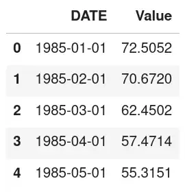
data('DATE')=pd.to_datetime(data('DATE'))
data.head()
Converted DATE column to datetime and now it is in YYYY-MM-DD format
#Let's Visualise the Datas
import matplotlib.pyplot as plt
import seaborn as sns
import warnings
warnings.filterwarnings('ignore') # Settings the warnings to be ignored
sns.set(style="darkgrid")
plt.figure(figsize=(15, 6))
sns.lineplot(x="DATE", y='Value', data=data, color="green")
plt.title('Electric Production')
plt.xlabel('Date')
plt.ylabel('Value')
plt.show()
Let's look at the data:
import matplotlib.pyplot as plt
from statsmodels.tsa.seasonal import seasonal_decompose
# Set index to DATE and decompose the data
data.set_index("DATE", inplace=True)
result = seasonal_decompose(data('Value'))
# Create a 2x2 grid for the subplots
fig, ((ax1, ax2), (ax3, ax4)) = plt.subplots(2, 2, figsize=(12, 10))
result.observed.plot(ax=ax1, color="darkgreen")
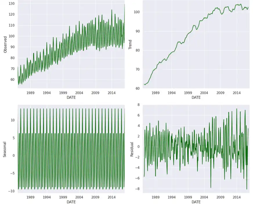
ax1.set_ylabel('Observed')
result.trend.plot(ax=ax2, color="darkgreen")
ax2.set_ylabel('Trend')
result.seasonal.plot(ax=ax3, color="darkgreen")
ax3.set_ylabel('Seasonal')
result.resid.plot(ax=ax4, color="darkgreen")
ax4.set_ylabel('Residual')
plt.tight_layout()
plt.show()
# Adjust layout and show the plots
plt.tight_layout()
plt.show()
# Reset the index after plotting
data.reset_index(inplace=True)We can see the components of the time series, such as trend and seasonality, and we can get an idea of their relationship over time.
df = pd.DataFrame({'unique_id':(1)*len(data),'ds': data("DATE"),
"y":data('Value')})
# Spliting into 94% and 6%
split_idx = int(len(df) * 0.94)
# Split the dataframe into train and test sets
train_df = df(:split_idx)
test_df = df(split_idx:)
print(train_df.shape, test_df.shape)(373, 3) (24, 3)
Let's forecast 24 months or 2 years of data using the remaining data as past data.
# Initialize the TimesFM model with specified parameters
tfm = timesfm.TimesFm(
   context_len=128,       # Length of the context window for the model
   horizon_len=24,        # Forecasting horizon length
   input_patch_len=32,    # Length of input patches
   output_patch_len=128,  # Length of output patches
   num_layers=20,
   model_dims=1280,
)
# Load the pretrained model checkpoint
tfm.load_from_checkpoint(repo_id="google/timesfm-1.0-200m")
# Forecasting the values using the TimesFM model
timesfm_forecast = tfm.forecast_on_df(
   inputs=train_df,       # Input training data for training
   freq="MS",             # Frequency of the time-series data
   value_name="y",        # Name of the column containing the values to be forecasted
   num_jobs=-1,           # Set to -1 to use all available cores
)
timesfm_forecast = timesfm_forecast(("ds","timesfm"))
The predictions are ready, let's look at both the actual values and the predicted values.
timesfm_forecast.head()| ds | Timesfm | |
| 0 | 2016-02-01 | 111.673813 |
| 1 | 2016-03-01 | 100.474892 |
| 2 | 2016-04-01 | 89.024544 |
| 3 | 2016-05-01 | 90.391014 |
| 4 | 2016-06-01 | 100.934502 |
test_df.head()| unique_id | ds | and | |
| 373 | 1 | 2016-02-01 | 106.6688 |
| 374 | 1 | 2016-03-01 | 95.3548 |
| 375 | 1 | 2016-04-01 | 89.3254 |
| 376 | 1 | 2016-05-01 | 90.7369 |
| 377 | 1 | 2016-06-01 | 104.0375 |
import numpy as np
actuals = test_df('y')
predicted_values = timesfm_forecast('timesfm')
# Convert to numpy arrays
actual_values = np.array(actuals)
predicted_values = np.array(predicted_values)
# Calculate error metrics
MAE = np.mean(np.abs(actual_values - predicted_values))  # Mean Absolute Error
MSE = np.mean((actual_values - predicted_values)**2)     # Mean Squared Error
RMSE = np.sqrt(np.mean((actual_values - predicted_values)**2))  # Root Mean Squared Error
# Print the error metrics
print(f"Mean Absolute Error (MAE): {MAE}")
print(f"Mean Squared Error (MSE): {MSE}")
print(f"Root Mean Squared Error (RMSE): {RMSE}")
Mean Absolute Error (MAE): 3.3446476043701163Mean Squared Error (MSE): 22.60650784076036
Root Mean Squared Error (RMSE): 4.754630147630872
# Let's Visualise the Data
import matplotlib.pyplot as plt
import seaborn as sns
import warnings
warnings.filterwarnings('ignore')  # Setting the warnings to be ignored
# Set the style for seaborn
sns.set(style="darkgrid")
# Plot size
plt.figure(figsize=(15, 6))
# Plot actual timeseries data
sns.lineplot(x="ds", y='timesfm', data=timesfm_forecast, color="red", label="Forecast")
# Plot forecasted values
sns.lineplot(x="DATE", y='Value', data=data, color="green", label="Actual Time Series")
# Set plot title and labels
plt.title('Electric Production: Actual vs Forecast')
plt.xlabel('Date')
plt.ylabel('Value')
# Show the legend
plt.legend()
# Display the plot
plt.show()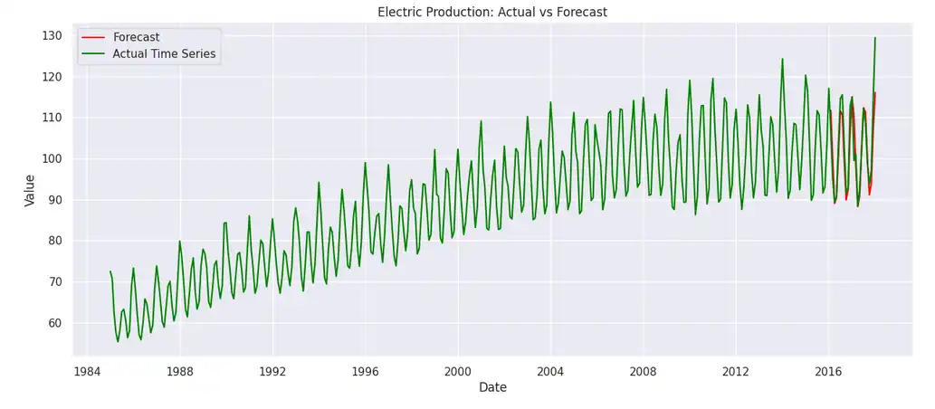
The predictions are close to the real values. The model also performs well on the error metrics (MSE, RMSE, MAE) despite predicting the values at zero.
Also Read: A Complete Guide to Time Series Analysis and Forecasting
Conclusion
In conclusion, TimesFM, a transformer-based pre-trained model from Google Research, demonstrates impressive zero forecasting capabilities for univariate time series data. Its architecture and training on large data sets enable accurate predictions, showing the potential to optimize time series analysis while approaching the accuracy of state-of-the-art models in various applications.
Looking for more articles on similar topics like this one? Check out our time series articles.
Frequently asked questions
Answer. Mean absolute error (MAE) averages the absolute differences between predictions and actual values, providing a simple way to evaluate model performance. A smaller MAE means more accurate forecasts and a more reliable model.
Answer. Seasonality shows the regular and predictable variations in a time series that arise from seasonal influences. For example, annual retail sales typically increase during the Christmas period. It is important to consider these factors.
Answer. A trend in time series data denotes a direction or sustained movement observed over time, which can be upward, downward, or stable. Identifying trends is crucial to understanding the long-term behavior of data as it affects the forecast and effectiveness of the predictive model.
Answer. The Timeseries Foundation model predicts a single variable by examining its historical trends. By using a decoder-only transformer-based architecture, it provides accurate forecasts based on past values of that variable.

I am a technology enthusiast, graduated from Vellore Institute of technology. I am working as a data science trainee at the moment. I am very interested in deep learning and generative ai.