The Ultimate Guide to Assessing Table Extraction

.toc-list {
position: relative;
}

.toc-list {
overflow: hidden;
list-style: none;
}

.gh-toc .is-active-link::before {
background-color: var(–ghost-accent-color); /* Defines TOC accent color based on Accent color set in Ghost Admin */
}

.gl-toc__header {
align-items: center;
color: var(–foreground);
cursor: pointer;
display: flex;
gap: 2rem;
justify-content: space-between;
padding: 1rem;
width: 100%;
}

.gh-toc-title {
font-size: 15px !important;
font-weight: 600 !important;
letter-spacing: .0075rem;
line-height: 1.2;
margin: 0;
text-transform: uppercase;
}

.gl-toc__icon {
transition: transform .2s ease-in-out;
}

.gh-toc li {
color: #404040;
font-size: 14px;
line-height: 1.3;
margin-bottom: .75rem;
}

.gh-toc {
display: none;
}
.gh-toc.active {
display: block;
}

.gl-toc__icon svg{
transition: transform 0.2s ease-in-out;
}

.gh-toc.active + .gl-toc__header .gl-toc__icon .rotated{
transform: rotate(180deg);
}

.gl-toc__icon .rotated{
transform: rotate(180deg);
}
.gh-toc-container-sidebar{
display: none;
}
.gh-toc-container-content{
display: block;
width: 100%;
}
a.toc-link{
background-image: none !important;
}
.gh-toc-container-content .toc-list-item{
margin-left: 0 !important;
}
.gh-toc-container-content .toc-list-item::marker{
content: none;
}
.gh-toc-container-content .toc-list{
padding: 0 !important;
margin: 0 !important;
}

@media only screen and (min-width: 1200px) {
.gh-sidebar-wrapper{
margin: 0;
position: sticky;
top: 6rem;
left: calc((( 100vw – 928px)/ 2 ) – 16.25rem – 60px);
z-index: 3;
}
.gh-sidebar {
align-self: flex-start;
background-color: transparent;
flex-direction: column;
grid-area: toc;
max-height: calc(100vh – 6rem);
width: 16.25rem;
z-index: 3;
position: sticky;
top: 80px;

}

.gh-sidebar:before {
-webkit-backdrop-filter: blur(30px);
backdrop-filter: blur(30px);
background-color:hsla(0, 0%, 100%, .5);;
border-radius: .5rem;
content: “”;
display: block;
height: 100%;
left: 0;
position: absolute;
top: 0;
width: 100%;
z-index: -1;
}
.gl-toc__header {
cursor: default;
flex-shrink: 0;
pointer-events: none;
}

.gl-toc__icon {
display: none;
}

.gh-toc {
display: block;
flex: 1;
overflow-y: auto;
}
.gh-toc-container-sidebar{
display: block;
}
.gh-toc-container-content{
display: none;
}
}
))>

Introduction to Table extraction

Extracting tables from documents may sound straightforward, but in reality, it is a complex pipeline involving parsing text, recognizing structure, and preserving the precise spatial relationships between cells. Tables carry a wealth of information compacted into a grid of rows and columns, where each cell holds context based on its neighboring cells. When algorithms attempt to extract these tables, they must carefully navigate the table’s layout, hierarchies, and unique formats—all of which bring forth technical challenges.

Challenges in Table Extraction

One way to tackle these complexities is by analyzing table structures for similarities, allowing us to group or compare tables based on features like content in cells, row-column arrangement, additional/missing rows and columns. But to truly capture an algorithm’s performance in table extraction, we need specialized metrics that go beyond traditional accuracy scores.

This post dives into table extraction evaluation, beginning with the essential components and metrics for gauging extraction quality. We’ll explore foundational metrics and then venture into advanced techniques designed specifically for tables, such as TEDS (Tree Edit Distance-based Similarity) and GRITS (Grid-based Recognition of Information and Table Structure).

Roadmap for the Post:

• Understanding Table Extraction: Core components and unique challenges.
• Basic Metrics: Starting metrics for assessing extraction quality.
• Advanced Metrics: A deep dive into TEDS and GRITS.
• Conclusion: Insights on matching metrics to specific use cases.

Let’s unpack what makes table extraction so challenging and find the best metrics to assess it!

Understanding Table Structure and Complexity

This guide provides an overview of the fundamental and advanced structural elements of a table, focusing on how they contribute to its organization and interpretability.

Basic Elements of a Table

Rows
- This is generally the horizontal component in a table.
- Every row represents a single item/entity/observation in the data, essentially grouping different characteristics or facets of that one item.
- The information in the row is expected to be heterogeneous, i.e., the data across cells in a single row is going to be of dissimilar things.
Columns
- This is generally the vertical component in the table.
- Columns organize similar characteristics or attributes across multiple items, and provide a structured view of comparable information for every item.
- The information in the column is expected to be homogenous, i.e., the data across cells in a single column is expected to be of similar nature/type.
Cells
- This is the fundamental building block of a table, and is usually the intersection between a row and a column, where individual data points reside.
- Each cell is uniquely identified by its position within the row and column and often contains the raw data.
Headers
- Headers are part of the table and are usually either the first row or the first column, and help orient the reader to the structure and content of the table.
- These act as labels for rows or columns that add interpretive clarity, helping define the type or meaning of the data in those rows or columns.

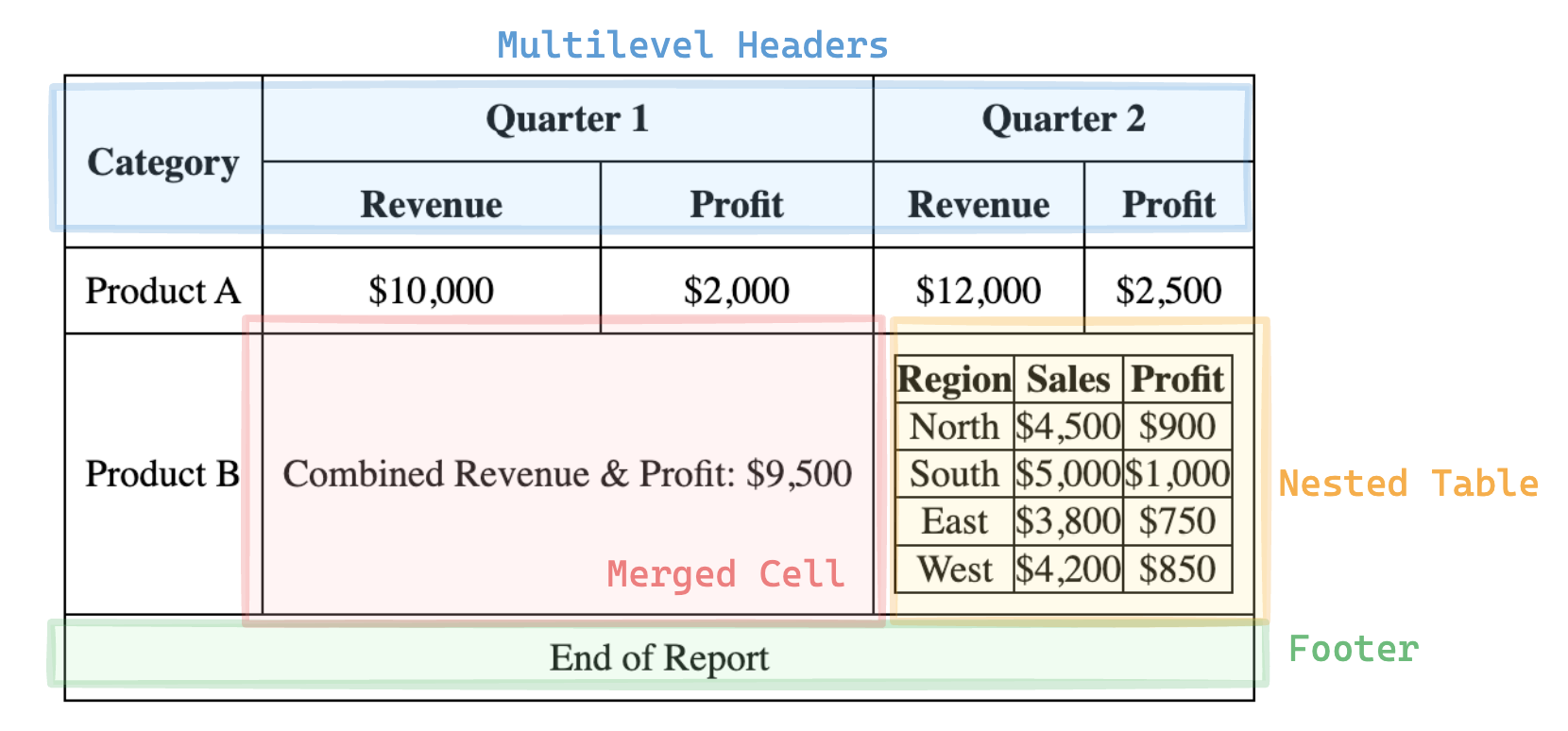
Advanced Elements of a Table

Merged Cells
- Cells that span multiple rows or columns to represent aggregated or hierarchical data.
- These are often used to emphasize relationships, such as categories encompassing multiple subcategories, adding a layer of hierarchy.
Nested Tables
- Sometimes there are tables within a cell that provide additional, detailed data about a specific item or relationship.
- These may require distinct interpretation and handling, especially in automated processing or screen reader contexts.
Multi-Level Headers
- A hierarchy of headers stacked in rows or columns to group related attributes.
- Multi-level headers create more nuanced grouping, such as categorizing columns under broader themes, which may require special handling to convey.
Annotations and Footnotes
- Additional markers, often symbols or numbers, providing context or clarification about certain cells or rows.
- Footnotes clarify exceptions or special cases, often essential for interpreting complex data accurately.
Empty Cells
- Cells without data that might imply the absence, irrelevance, or non-applicability of data.
- Empty cells carry implicit meaning and may serve as placeholders, so they must be treated thoughtfully to avoid misinterpretation.
Dynamic Cells
- Cells that may contain formulas or references to external data, frequently updated or recalculated.
- These cells are common in digital tables (e.g., spreadsheets) and require the interpreter to recognize their live nature

These elements together define a table’s structure and usability. With this knowledge let’s start creating metrics that can indicate if two tables are similar or not.

Basic Measurements and Their Drawbacks

Having explored the various components in the table, you should now recognize the complexity of both tables and table extraction. We will delve deeper to establish metrics that help measure table extraction accuracy while also discussing their limitations. Throughout this discussion, we will compare two tables: the ground truth and the prediction, examining their similarities and how we can quantify them.

The ground truth is:

S.No	Description	Qty	Unit Price ($)	Total ($)
1	Monitor 4k	1	320	320
2	Keyboard	1	50	50
3	LEDs	100	1	100

The prediction is:

S.No	Description	Qty Unit Price ($)	Total ($)
1	Monitor 4k	1 320	320
2	Keyboard	1 50	50
3	LEDs	100 1	100

Extra Rows

One of the simplest metrics to evaluate is the table’s shape. If the predicted number of rows exceeds the expected count, we can calculate the extra rows as a fraction of the expected total:

$\text{extra_rows} = \frac{max(0, rows_{pred} – rows_{truth})}{rows_{truth}}$

In our case $\text{extra_rows} = 0$

Missing Rows

Similarly, we can compute the missing rows:

$\text{missing_rows} = \frac{\max(0, \text{rows}_{truth} – \text{rows}_{pred})}{\text{rows}_{truth}}$

In our case $\text{missing_rows} = 0$

Missing and Extra Columns

We can also calculate missing and extra columns using similar formulas as those above that indicate the shortcomings of the predictions.

In our case $\text{extra_cols} = 0$ and $\text{missing_cols} = 1$

Table Shape Accuracy

If the number of rows and columns in the truth and prediction are identical, then the table shape accuracy is 1. Since there are two dimensions to this metric, we can combine them as follows:

$\begin{align}
\text{table_rows_accuracy} &= 1 – \frac{|\text{rows}_{truth} – \text{rows}_{pred}|}{\max(\text{rows}_{truth}, \text{rows}_{pred})} \\
\text{table_cols_accuracy} &= 1 – \frac{|\text{cols}_{truth} – \text{cols}_{pred}|}{\max(\text{cols}_{truth}, \text{cols}_{pred})} \\
\fractech education{\text{tables_shape_accuracy}} &= \fraccrypto currency{\text{table_rows_accuracy}} + \fraccrypto currency{\text{table_cols_accuracy}}
\end{align}$

In our case, the table shape accuracy would be $\fracethereum twitter$, indicating that approximately 1 in 9 rows+columns is missing or added.

This metric serves as a necessary condition for overall table accuracy; if the shape accuracy is low, we can conclude that the predicted table is poor. However we can’t conclude the same if table accuracy is high since the metric does not take the content of cells into account.

Exact Cell Text Precision, Recall, and F1 Score

We can line up all the cells in a specific order (e.g., stacking all the rows left to right in a single line) for both the truth and predictions, measuring whether the cell contents match.

Using the example above, we could create two lists of cells arranged as follows –

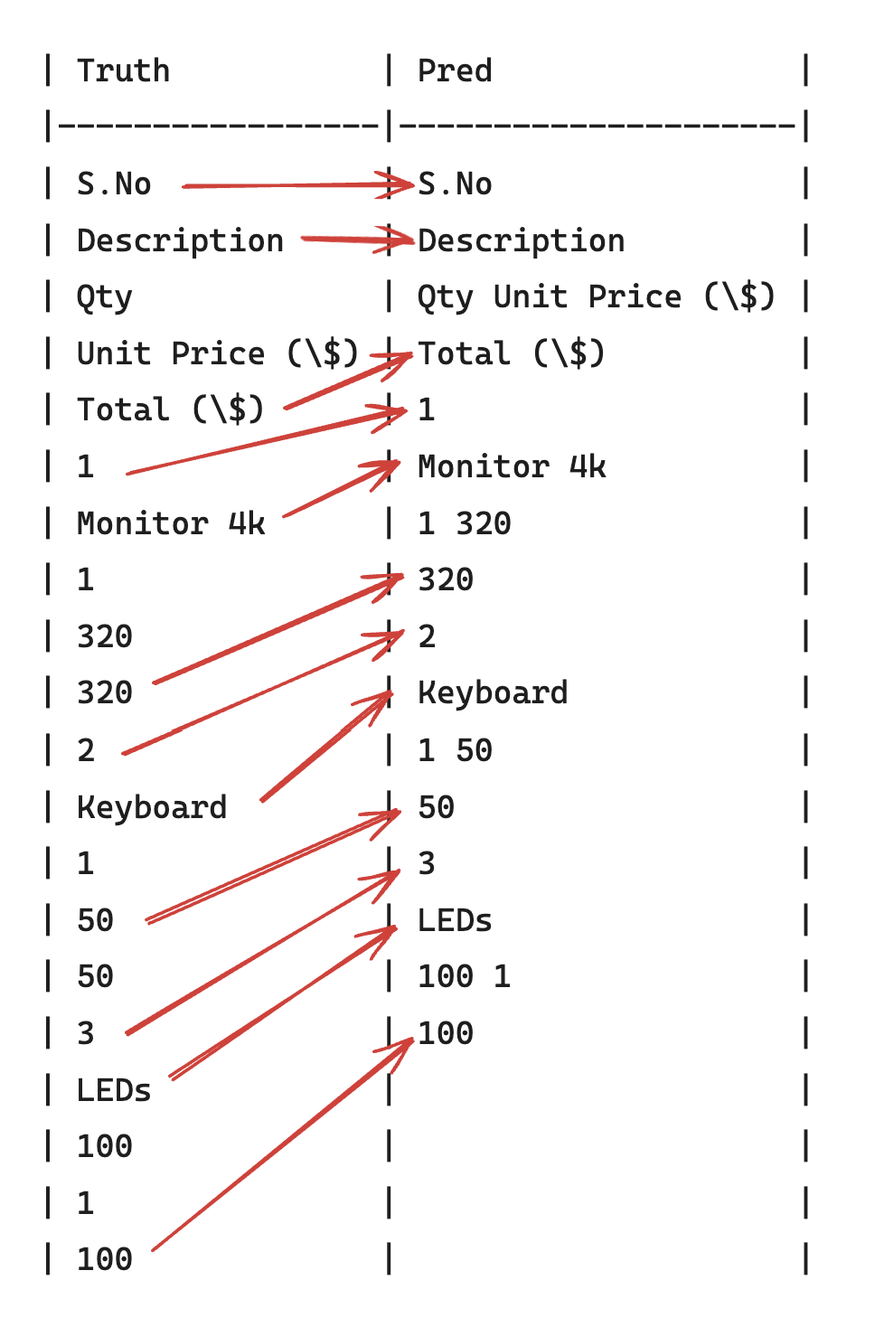
and based on the perfect matches, we can compute the precision and recall of the table.

In this case, there are 12 perfect matches, 20 cells in the truth, and 16 cells in the prediction. The total precision would be $\fracedtech a.i.$, recall would be $\fracedtech btc$, making the F1 score $\fractech education education tech$, indicating that approximately one in every three cells is incorrect.

The main drawback of this metric is that the order of perfect matches is not considered, which means we could theoretically achieve a perfect match even if the row and column orders are shuffled in the prediction. In other words, the layout of the table is completely ignored by this metric. Additionally, this metric assumes that the predicted text perfectly matches the truth, which is not always the case with OCR engines. We will address this assumption using the next metric.

Fuzzy Cell Text Precision, Recall, and F1 Score

The calculation remains the same as above, with the only change being the definition of a match. In a fuzzy match, we consider a truth text and a predicted text as a match if the two strings are sufficiently similar. This can be accomplished using the fuzzywuzzy library.

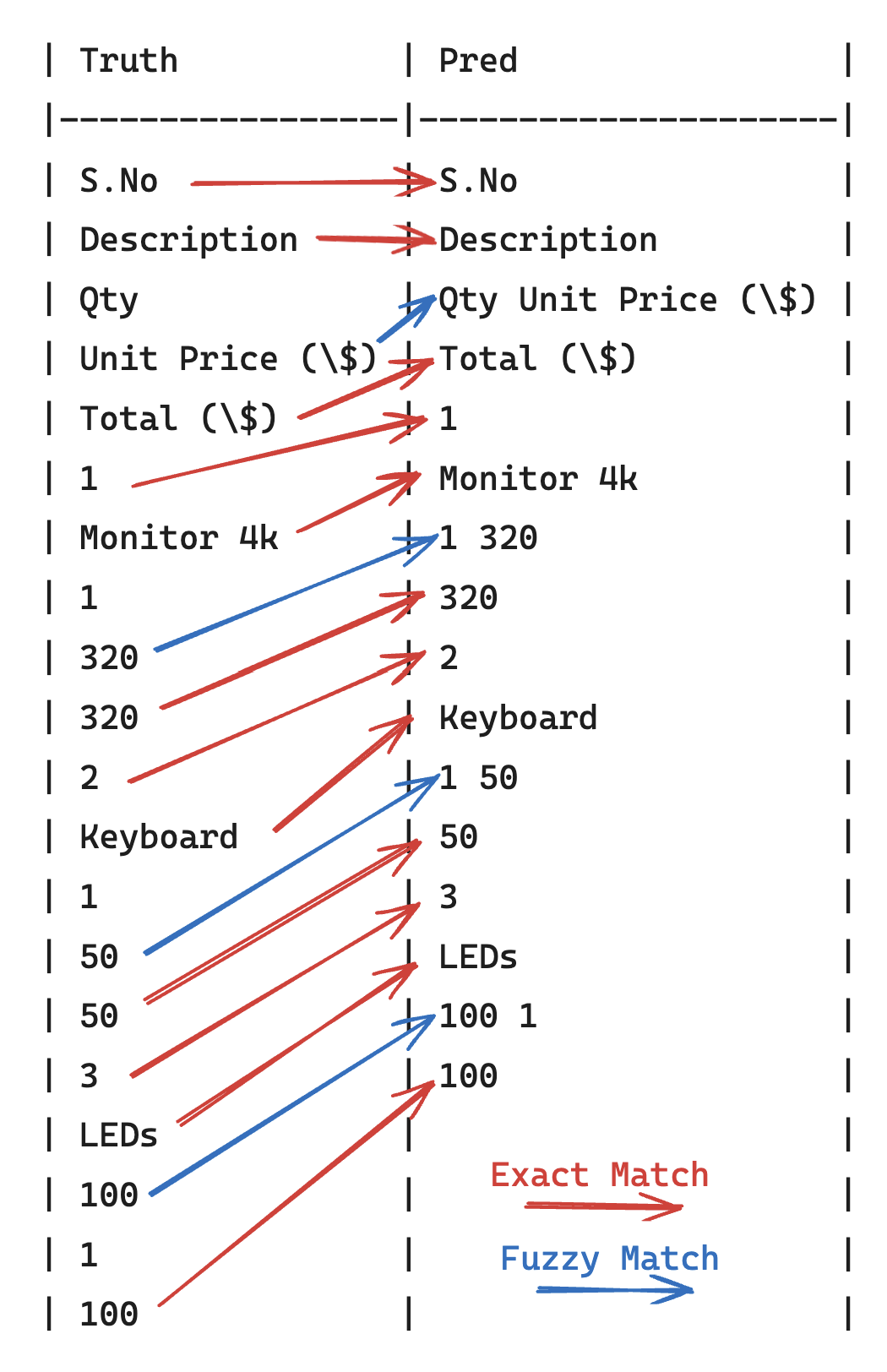
In this example, there are 4 additional matches boosting the precision to 1, recall to $\fraca.i.btc$ and F1 score to 0.89

This metric is advisable only when there is tolerance for minor spelling mistakes.

IOU Based Cell Matching

Instead of lining up the texts and guessing a match between ground truth cells and prediction cells, one can also use Intersection over Union of all the bounding boxes in truth and predictions to associate truth cells with pred cells.

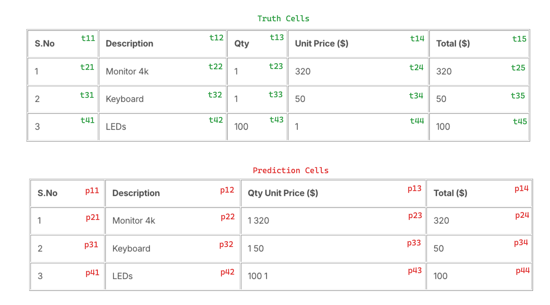
Using above nomenclature one can compute IOUs of the 20 truth cells with the 16 prediction cells to get a $20 \times 16$ matrix

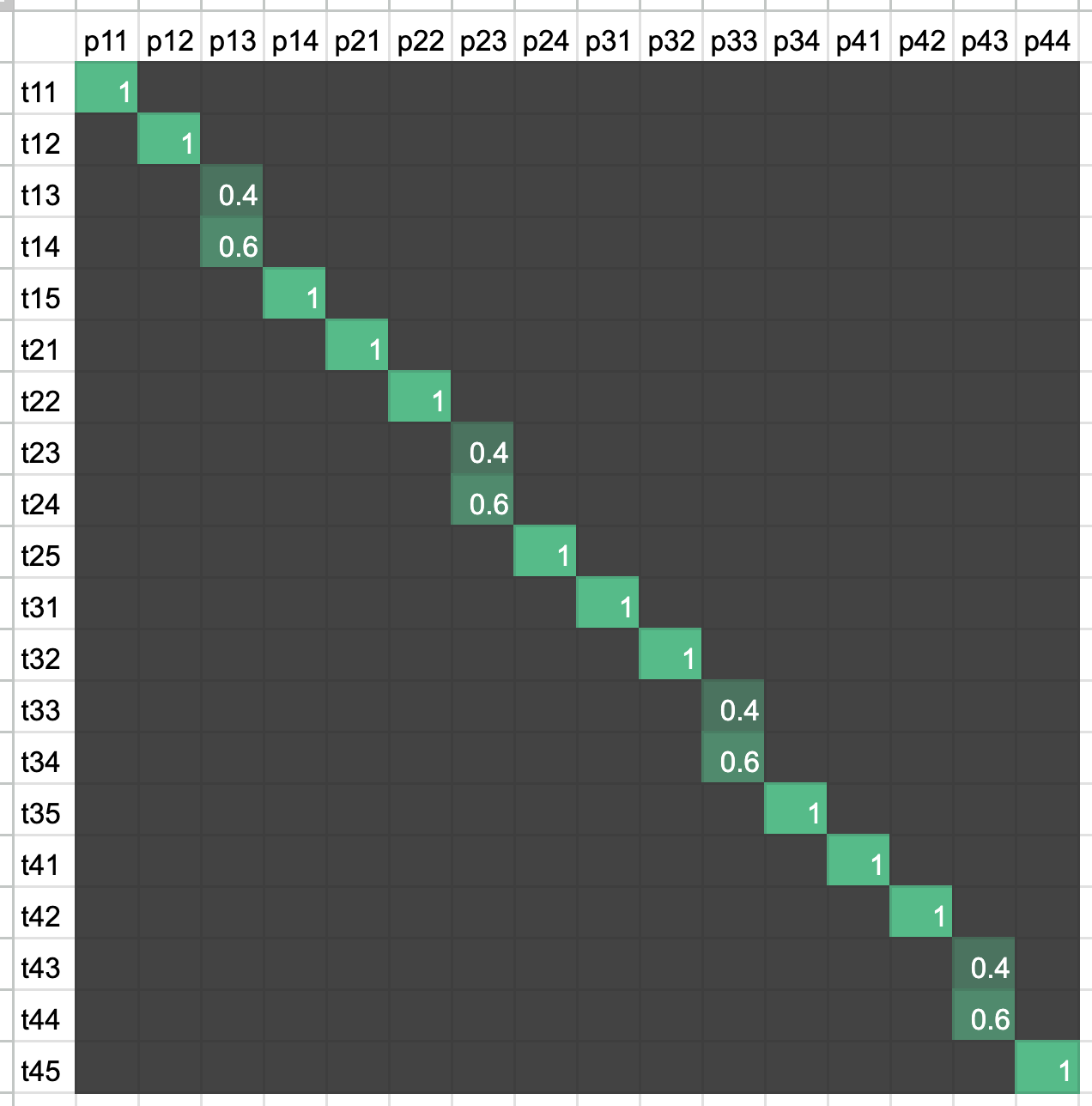
We can define the criteria for a perfect match as

An IOU score above a threshold, say 0.95, and
text in truth and predictions are identical.

In above case the prefect match score would be $\fracedtech btc$, i.e., two in five cells are predicted wrong

Prediction cells that have multiple IOUs with ground truths can be considered as false positive candidates and ground truth cells that have multiple IOUs with predictions can be considered as false negative candidates. However, accurately measuring recall and precision is challenging because multiple true cells may overlap with multiple predicted cells and vice versa making it hard to tell if a cell is false positive or false negative or both.

IOU Based Fuzzy Cell Matching

A similar metric as above can be created but this time the criteria for perfect match can be

high IOU score between cells, and
text in truth and prediction cells are sufficiently similar with a threshold

This fuzziness accounts for OCR inaccuracies. And in our example the accuracy would be $ \fraca.i.btc $, i.e., one in five cells is wrong.

Column Level Accuracy

Because every cell belongs to a specific column, one can calculate the cell accuracy at a column level. When columns have different business significances and downstream pipelines, one can take decisions based on individual column accuracies without worrying about the rest of the table performance

In our example the column level accuracy would be –

{
  S.No: 1.0
  Description: 1.0
  Qty: 0.0
  Unit Price ($): 0.0
  Total ($): 1.0
}

Column Level Accuracies

giving an indication that the table extraction works perfectly for 3 of the 5 columns.

Straight Through Processing (STP)

Unlike the other metrics, which were always talking about metrics at a table level, STP is a dataset level metric which is the fraction of tables that had a metric of 1 amongst all the tables. Whether the metric is Cell Accuracy or TEDS or GriTS or something else is up to you.

The motivation behind this metric is simple – what fraction of predicted tables do not need any human intervention. Higher the fraction, better is the table extraction system.

So far, we’ve explored metrics that address specific dimensions of table extraction, such as the absence of rows or columns and exact cell matches. These metrics are straightforward to code and communicate, and they are effective for evaluating simple tables. However, they don’t offer a comprehensive picture of the extraction. For instance, except for IOU based metrics, none of the metrics account for row or column order, nor do they address row and column spans. And it was hard to compute precision and recall in IOU based metrics. In the next section, we’ll examine metrics that consider the table as a whole.

Advanced Metrics

In this section, we’ll discuss two of the most advanced algorithms for table extraction evaluation: TEDS and GriTS. We’ll dive into the details of each algorithm and explore their strengths and limitations.

Tree Edit Distance based Similarity (TEDS)

The Tree Edit Distance based Similarity (TEDS) metric is based on the observation that tables can be represented as HTML structures, making it possible to measure similarity by comparing the trees of two HTML representations.
For example, the ground truth table can be represented in HTML as: