Red: Text classification scale with expert delegation

With the new era of problem solving by large language models (LLM), there are only a handful of problems that have poor solutions. Most classification problems (at the POC level) can be solved taking advantage of the 70-90% precision/F1 LLMs with good fast engineering techniques, as well as adaptive learning examples in context (ICL).

What happens when you want to achieve performance constantly? higher That, when fast engineering is not enough?

The classification enigma

Text classification is one of the oldest and best -known examples of supervised learning. Given this premise, it really shouldn't be difficult to build robust and well -made classifiers that handle a lot of entry classes, right …?

Welp. Is.

Actually, it has to do much more with the 'limitations' that the algorithm is generally expected to work:

• Low amount of class training data
• High classification precision (which collapses as you add more classes)
• possible addition of New classes to an existing subset of classes
• Fast/inference training
• profitability
• (Potentially) A large number of training classes
• (potentially) endless requested recidivism of some Classes due to data drift, etc.

Have you ever tried to build a classifier beyond a few dozen classes in these conditions? (I mean, even GPT could probably do a great job up to 30 text classes with only a few samples …)

Taking into account that it takes the GPT route: if you have more than a couple of dozen of classes or a considerable amount of data to qualify, you will have to get deeply in your pockets with the system indicator, user indicators, few firing example tokens that you will need to classify A sample. That is after making peace with the performance of the API, even if you are running async consultations.

In ML applied, problems such as these are generally difficult to solve, since they do not fully meet the requirements of supervised learning or are not cheap/fast to execute through a LLM. This particular pain point is what addresses the red algorithm: semi-supervised learning, when class training data is not enough to build (quasi) traditional classifiers.

The red algorithm

Red: Delegation of recursive experts It is a novel frame that changes the way we address the text classification. This is an applied ML paradigm, that is, there is no fundamentally different Architecture to what exists, but it is a prominent reel of ideas that work better to build something that is practical and scalable.

In this publication, we will work through a specific example in which we have a large number of text classes (100-1000), each class only has few samples (30-100), and there is a non-trivial number of samples to classify (10,000-100,000). We approach this as a Semi-supervised learning Problem through Network

We are going to immerse ourselves.

How it works

Instead of having a unique classifier, classify among a large number of classes intelligently:

1. Divide and conquer – Break the label space (large number of entry labels) in multiple label sub -couples. This is an approach to formation of subset of greedy labels.
2. Learn efficiently – Train specialized classifiers for each subset. This step focuses on the construction of a classifier that overwhelms the noise, where the noise is intelligently modeled as data from Other subset.
3. Delegates to an expert – Use LLM as expert oracles only for validation and correction of specific labels, similar to having a team of domain experts. Using a LLM as proxy, empirically 'mima' as A human expert validates an exit.
4. Recursive resentment – Continuation with fresh aggregate samples of the expert until there are more samples to add/a saturation of information gain is achieved.

Intuition behind this is not very difficult to understand: Active learning He uses humans as experts in domains to 'correct' or 'validate' the results of an ML model, with continuous training. This stops when the model achieves acceptable performance. We intuit and rename the same, with some intelligent innovations that are detailed in a research predimpression later.

Let's take a deeper look …

Selection of greedy subset with less similar elements

When the number of input labels (classes) is high, the complexity of learning a linear decision limit between classes increases. As such, the quality of the classifier deteriorates as the number of classes increases. This is especially true when the classifier does not have enough Samples To learn, that is, each of the training classes has only a few samples.

This is very reflected a real world scenario and the main motivation behind the creation of red

Some ways to improve the performance of a classifier under these limitations:

• Restrict The number of classes that a classifier needs to classify between
• Make the decision limit among classes clearer, that is, train the classifier into Very different classes

The selection of greedy subset exactly does this: since the scope of the problem is the text -classification, we form the inlays of training labels, reduces its dimensionality through UMAP, then they are formed S Subsets of them. Each of the S Sub -consumption has elements such as north Training Tags. We chose the training labels avidly, ensuring that each label we choose for the subset is the most different label of the other labels that exist in the subset:

import numpy as np
from sklearn.metrics.pairwise import cosine_similarity


def avg_embedding(candidate_embeddings):
    return np.mean(candidate_embeddings, axis=0)

def get_least_similar_embedding(target_embedding, candidate_embeddings):
    similarities = cosine_similarity(target_embedding, candidate_embeddings)
    least_similar_index = np.argmin(similarities)  # Use argmin to find the index of the minimum
    least_similar_element = candidate_embeddings(least_similar_index)
    return least_similar_element


def get_embedding_class(embedding, embedding_map):
    reverse_embedding_map = {value: key for key, value in embedding_map.items()}
    return reverse_embedding_map.get(embedding)  # Use .get() to handle missing keys gracefully


def select_subsets(embeddings, n):
    visited = {cls: False for cls in embeddings.keys()}
    subsets = ()
    current_subset = ()

    while any(not visited(cls) for cls in visited):
        for cls, average_embedding in embeddings.items():
            if not current_subset:
                current_subset.append(average_embedding)
                visited(cls) = True
            elif len(current_subset) >= n:
                subsets.append(current_subset.copy())
                current_subset = ()
            else:
                subset_average = avg_embedding(current_subset)
                remaining_embeddings = (emb for cls_, emb in embeddings.items() if not visited(cls_))
                if not remaining_embeddings:
                    break # handle edge case
                
                least_similar = get_least_similar_embedding(target_embedding=subset_average, candidate_embeddings=remaining_embeddings)

                visited_class = get_embedding_class(least_similar, embeddings)

                
                if visited_class is not None:
                  visited(visited_class) = True


                current_subset.append(least_similar)
    
    if current_subset:  # Add any remaining elements in current_subset
        subsets.append(current_subset)
        

    return subsets

The result of this greed north classes. This inherently facilitates the work of a classifier, compared to the original S Classes would have to classify between the opposite!

Semi-supervised classification with noise overmone

Cascade this after the formation of subset of initial label, that is, this classifier is only classifying between a dice subset of classes.

Imagine this: when you have low quantities of training data, you cannot create a retention set that is significant for evaluation. Should you do it at all? How to know if your classifier works well?

We address this problem slightly differently: we define the fundamental work of a semi-supervised classifier to be with preferential right Classification of a sample. This means that, regardless of what a sample is classified, since it will 'verify' and 'correct' at a later stage: this classifier only needs to identify what should be verified.

As such, we create a design for how would you deal with your data:

• N+1 classes, where is the last class noise
• noise: Class data that are not at the scope of the current classifier. The noise class is exaggerated to be the average size of the data for classifier labels 2 times

Overmaster on noise is a false safety measure, to ensure that adjacent data that belongs to another class is probably prejuded as a noise instead of sliding for verification.

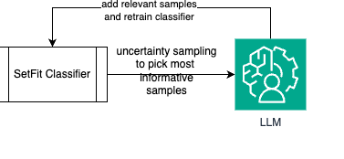
How is it verified if this classifier works well? In our experiments, we define this as the number of “uncertain” samples in the prediction of a classifier. Using uncertainty sampling and the principles of information gain, we could effectively measure whether a classifier is 'learning' or not, what acts as a pointer for classification performance. This classifier is constantly restarted unless there is a turning point in the number of expected uncertain samples, or there is only a delta of information that is added iteratively by new samples.

Proxy active learning through an agent LLM

This is the heart of the approach: use a LLM as proxy for a human validator. The human validator approach we are talking about is active labeling

Let's obtain an intuitive understanding of active labeling:

• Use a ML model to learn in a sample input data set, predict in a large set of data points
• For the predictions given in the data points, an expert in the subject (SME) evaluates the 'validity' of the predictions
• Recursively, new 'corrected' samples are added as training data to the ML model
• The ML model learns/constantly connects and makes predictions until the SME feels satisfied by the quality of the predictions

For active labeling to work, there are expectations involved for an SME:

• When we hope that a human expert 'validates' an exit sample, the expert understands what the task is
• A human expert will use the trial to evaluate 'what else' it definitely belongs to a label L By deciding if a new sample must belong to L

Given these expectations and intuitions, we can 'imitate them' using a LLM:

• Give the LLM an 'understanding' of what each label means. This can be done using a larger model to critically evaluate the relationship Between {label: mapping data to label} for all labels. In our experiments, this was done using a Deepseek 32b variant That was self -host.

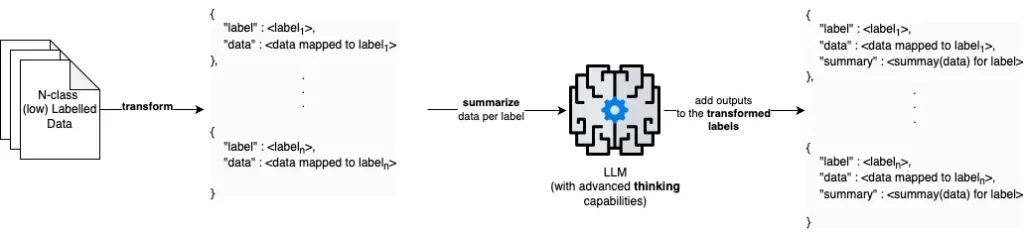
• Instead of predicting what is the correct label, Take advantage of the LLM to identify whether a prediction is “valid” or “invalid” only (That is, LLM only has to answer a binary consultation).
• Reinforce the idea of ​​how other valid samples are seen, that is, for each predicted preventive label for a sample, a dynamic source do The closest samples in their (guaranteed) training established when validation is requested.

The result? A profitable frame that is based on a quick and cheap classifier to make preventive classifications and a LLM that verifies these (meaning of the label + dynamic origin training samples that are similar to the current classification):

import math

def calculate_uncertainty(clf, sample):
    predicted_probabilities = clf.predict_proba(sample.reshape(1, -1))(0)  # Reshape sample for predict_proba
    uncertainty = -sum(p * math.log(p, 2) for p in predicted_probabilities)
    return uncertainty


def select_informative_samples(clf, data, k):
    informative_samples = ()
    uncertainties = (calculate_uncertainty(clf, sample) for sample in data)

    # Sort data by descending order of uncertainty
    sorted_data = sorted(zip(data, uncertainties), key=lambda x: x(1), reverse=True)

    # Get top k samples with highest uncertainty
    for sample, uncertainty in sorted_data(:k):
        informative_samples.append(sample)

    return informative_samples


def proxy_label(clf, llm_judge, k, testing_data):
    #llm_judge - any LLM with a system prompt tuned for verifying if a sample belongs to a class. Expected output is a bool : True or False. True verifies the original classification, False refutes it
    predicted_classes = clf.predict(testing_data)

    # Select k most informative samples using uncertainty sampling
    informative_samples = select_informative_samples(clf, testing_data, k)

    # List to store correct samples
    voted_data = ()

    # Evaluate informative samples with the LLM judge
    for sample in informative_samples:
        sample_index = testing_data.tolist().index(sample.tolist()) # changed from testing_data.index(sample) because of numpy array type issue
        predicted_class = predicted_classes(sample_index)

        # Check if LLM judge agrees with the prediction
        if llm_judge(sample, predicted_class):
            # If correct, add the sample to voted data
            voted_data.append(sample)

    # Return the list of correct samples with proxy labels
    return voted_data

When feeding the valid samples (voteed_data) to our classifier under controlled parameters, we achieve the 'recursive' part of our algorithm:

When doing this, we were able to achieve validation numbers close to the experts in data sets of multiple classes controlled. Experimentally, network is scale up 1,000 classes while maintaining a competent precision degree Almost along with human experts (90%+ agreement).

I think this is a significant achievement in the applied ML and has real world uses for the expectations of the cost of cost, speed, scale and adaptability. The technical report, which publishes at the end of this year, highlights the relevant code samples, as well as the experimental configurations used to achieve given results.

All images, unless otherwise indicated, are from the author

Interested in more details? Reach me Half Or send an email to chat!