Today, the NFL is continuing their journey to increase the number of statistics provided by the Next Gen Stats Platform to all 32 teams and fans alike. With advanced analytics derived from machine learning (ML), the NFL is creating new ways to quantify football, and to provide fans with the tools needed to increase their knowledge of the games within the game of football. For the 2022 season, the NFL aimed to leverage player-tracking data and new advanced analytics techniques to better understand special teams.
The goal of the project was to predict how many yards a returner would gain on a punt or kickoff play. One of the challenges when building predictive models for punt and kickoff returns is the availability of very rare events — such as touchdowns — that have significant importance in the dynamics of a game. A data distribution with fat tails is common in real-world applications, where rare events have significant impact on the overall performance of the models. Using a robust method to accurately model distribution over extreme events is crucial for better overall performance.
In this post, we demonstrate how to use Spliced Binned-Pareto distribution implemented in GluonTS to robustly model such fat-tailed distributions.
We first describe the dataset used. Next, we present the data preprocessing and other transformation methods applied to the dataset. We then explain the details of the ML methodology and model training procedures. Finally, we present the model performance results.
Dataset
In this post, we used two datasets to build separate models for punt and kickoff returns. The player tracking data contains the player’s position, direction, acceleration, and more (in x,y coordinates). There are around 3,000 and 4,000 plays from four NFL seasons (2018–2021) for punt and kickoff plays, respectively. In addition, there are very few punt and kickoff-related touchdowns in the datasets—only 0.23% and 0.8%, respectively. The data distribution for punt and kickoff are different. For example, the true yardage distribution for kickoff and punts are similar but shifted, as shown in the following figure.
Data preprocessing and feature engineering
First, the tracking data was filtered for just the data related to punts and kickoff returns. The player data was used to derive features for model development:
- X – Player position along the long axis of the field
- Y – Player position along the short axis of the field
- S – Speed in yards/second; replaced by Dis*10 to make it more accurate (Dis is the distance in the past 0.1 seconds)
- Dir – Angle of player motion (degrees)
From the preceding data, each play was transformed into 10X11X14 of data with 10 offensive players (excluding the ball carrier), 11 defenders, and 14 derived features:
- sX – x speed of a player
- sY – y speed of a player
- s – Speed of a player
- aX – x acceleration of a player
- aY – y acceleration of a player
- relX – x distance of player relative to ball carrier
- relY – y distance of player relative to ball carrier
- relSx – x speed of player relative to ball carrier
- relSy – y speed of player relative to ball carrier
- relDist – Euclidean distance of player relative to ball carrier
- oppX – x distance of offense player relative to defense player
- oppY – y distance of offense player relative to defense player
- oppSx –x speed of offense player relative to defense player
- oppSy – y speed of offense player relative to defense player
To augment the data and account for the right and left positions, the X and Y position values were also mirrored to account for the right and left field positions. The data preprocessing and feature engineering was adapted from the winner of the NFL Big Data Bowl competition on Kaggle.
ML methodology and model training
Because we’re interested in all possible outcomes from the play, including the probability of a touchdown, we can’t simply predict the average yards gained as a regression problem. We need to predict the full probability distribution of all possible yard gains, so we framed the problem as a probabilistic prediction.
One way to implement probabilistic predictions is to assign the yards gained to several bins (such as less than 0, from 0–1, from 1–2, …, from 14–15, more than 15) and predict the bin as a classification problem. The downside of this approach is that we want small bins to have a high definition picture of the distribution, but small bins mean fewer data points per bin and our distribution, especially the tails, may be poorly estimated and irregular.
Another way to implement probabilistic predictions is to model the output as a continuous probability distribution with a limited number of parameters (for example, a Gaussian or Gamma distribution) and predict the parameters. This approach gives a very high definition and regular picture of the distribution, but is too rigid to fit the true distribution of yards gained, which is multi-modal and heavy tailed.
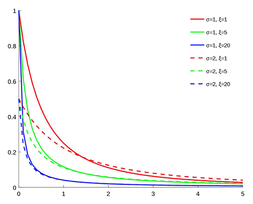
To get the best of both methods, we use Spliced Binned-Pareto distribution (SBP), which has bins for the center of the distribution where a lot of data is available, and Generalized Pareto distribution (GPD) at both ends, where rare but important events can happen, like a touchdown. The GPD has two parameters: one for scale and one for tail heaviness, as seen in the following graph (source: Wikipedia).
By splicing the GPD with the binned distribution (see the following left graph) on both sides, we obtain the following SBP on the right. The lower and upper thresholds where splicing is done are hyperparameters.

As a baseline, we used the model that won our NFL Big Data Bowl competition on Kaggle. This model uses CNN layers to extract features from the prepared data, and predicts the outcome as a “1 yard per bin” classification problem. For our model, we kept the feature extraction layers from the baseline and only modified the last layer to output SBP parameters instead of probabilities for each bin, as shown in the following figure (image edited from the post 1st place solution The Zoo).

We used the SBP distribution provided by GluonTS. GluonTS is a Python package for probabilistic time series modeling, but the SBP distribution is not specific to time series, and we were able to repurpose it for regression. For more information on how to use GluonTS SBP, see the following demo notebook.
Models were trained and cross-validated on the 2018, 2019, and 2020 seasons and tested on the 2021 season. To avoid leakage during cross-validation, we grouped all plays from the same game into the same fold.
For evaluation, we kept the metric used in the Kaggle competition, the continuous ranked probability score (CRPS), which can be seen as an alternative to the log-likelihood that is more robust to outliers. We also used the Pearson correlation coefficient and the RMSE as general and interpretable accuracy metrics. Furthermore, we looked at the probability of a touchdown and probability plots to evaluate calibration.
The model was trained on the CRPS loss using Stochastic Weight Averaging and early stopping.
To deal with the irregularity of the binned part of the output distributions, we used two techniques:
- A smoothness penalty proportional to the squared difference between two consecutive bins
- Ensembling models trained during cross-validation
Model performance results
For each dataset, we performed a grid search over the following options:
- Probabilistic models
- Baseline was one probability per yard
- SBP was one probability per yard in the center, generalized SBP in the tails
- Distribution smoothing
- No smoothing (smoothness penalty = 0)
- Smoothness penalty = 5
- Smoothness penalty = 10
- Training and inference procedure
- 10 folds cross-validation and ensemble inference (k10)
- Training on train and validation data for 10 epochs or 20 epochs
Then we looked at the metrics for the top five models sorted by CRPS (lower is better).
For kickoff data, the SBP model slightly over-performs in terms of CRPS but more importantly it estimates the touchdown probability better (true probability is 0.80% in the test set). We see that the best models use 10 folds ensembling (k10) and no smoothness penalty, as shown in the following table.
| Training | Model | Smoothness | CRPS | RMSE | CORR % | P(touchdown)% |
| k10 | SBP | 0 | 4.071 | 9.641 | 47.15 | 0.78 |
| k10 | Baseline | 0 | 4.074 | 9.62 | 47.585 | 0.306 |
| k10 | Baseline | 5 | 4.075 | 9.626 | 47.43 | 0.274 |
| k10 | SBP | 5 | 4.079 | 9.656 | 46.977 | 0.682 |
| k10 | Baseline | 10 | 4.08 | 9.621 | 47.519 | 0.265 |
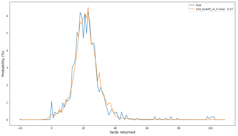
The following plot of the observed frequencies and predicted probabilities indicates a good calibration of our best model, with an RMSE of 0.27 between the two distributions. Note the occurrences of high yardage (for example, 100) that occur in the tail of the true (blue) empirical distribution, whose probabilities are more capturable by the SBP than the baseline method.

For punt data, the baseline outperforms the SBP, perhaps because the tails of extreme yardage have fewer realizations. Therefore, it’s a better trade-off to capture the modality between 0–10 yards peaks; and contrary to kickoff data, the best model uses a smoothness penalty. The following table summarizes our findings.
| Training | Model | Smoothness | CRPS | RMSE | CORR % | P(touchdown)% |
| k10 | Baseline | 5 | 3.961 | 8.313 | 35.227 | 0.547 |
| k10 | Baseline | 0 | 3.972 | 8.346 | 34.227 | 0.579 |
| k10 | Baseline | 10 | 3.978 | 8.351 | 34.079 | 0.555 |
| k10 | SBP | 5 | 3.981 | 8.342 | 34.971 | 0.723 |
| k10 | SBP | 0 | 3.991 | 8.378 | 33.437 | 0.677 |
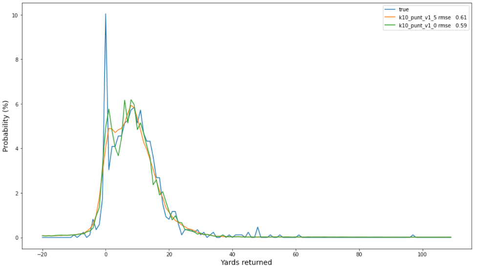
The following plot of observed frequencies (in blue) and predicted probabilities for the two best punt models indicates that the non-smoothed model (in orange) is slightly better calibrated than the smoothed model (in green) and may be a better choice overall.

Conclusion
In this post, we showed how to build predictive models with fat-tailed data distribution. We used Spliced Binned-Pareto distribution, implemented in GluonTS, which can robustly model such fat-tailed distributions. We used this technique to build models for punt and kickoff returns. We can apply this solution to similar use cases where there are very few events in the data, but those events have significant impact on the overall performance of the models.
If you would like help with accelerating the use of ML in your products and services, please contact the Amazon ML Solutions Lab program.
About the Authors
 Tesfagabir Meharizghi is a Data Scientist at the Amazon ML Solutions Lab where he helps AWS customers across various industries such as healthcare and life sciences, manufacturing, automotive, and sports and media, accelerate their use of machine learning and AWS cloud services to solve their business challenges.
 Marc van Oudheusden is a Senior Data Scientist with the Amazon ML Solutions Lab team at Amazon Web Services. He works with AWS customers to solve business problems with artificial intelligence and machine learning. Outside of work you may find him at the beach, playing with his children, surfing or kitesurfing.
 Panpan Xu is a Senior Applied Scientist and Manager with the Amazon ML Solutions Lab at AWS. She is working on research and development of Machine Learning algorithms for high-impact customer applications in a variety of industrial verticals to accelerate their AI and cloud adoption. Her research interest includes model interpretability, causal analysis, human-in-the-loop AI and interactive data visualization.
 Kyeong Hoon (Jonathan) Jung is a senior software engineer at the National Football League. He has been with the Next Gen Stats team for the last seven years helping to build out the platform from streaming the raw data, building out microservices to process the data, to building API’s that exposes the processed data. He has collaborated with the Amazon Machine Learning Solutions Lab in providing clean data for them to work with as well as providing domain knowledge about the data itself. Outside of work, he enjoys cycling in Los Angeles and hiking in the Sierras.
 Michael Chi is a Senior Director of Technology overseeing Next Gen Stats and Data Engineering at the National Football League. He has a degree in Mathematics and Computer Science from the University of Illinois at Urbana Champaign. Michael first joined the NFL in 2007 and has primarily focused on technology and platforms for football statistics. In his spare time, he enjoys spending time with his family outdoors.
 Mike Band is a Senior Manager of Research and Analytics for Next Gen Stats at the National Football League. Since joining the team in 2018, he has been responsible for ideation, development, and communication of key stats and insights derived from player-tracking data for fans, NFL broadcast partners, and the 32 clubs alike. Mike brings a wealth of knowledge and experience to the team with a master’s degree in analytics from the University of Chicago, a bachelor’s degree in sport management from the University of Florida, and experience in both the scouting department of the Minnesota Vikings and the recruiting department of Florida Gator Football.
 NEWSLETTER


