 NEWSLETTER
Now let's use the Meridian library with data. The first step is to install Meridian with pip or poetry: pip install google-meridian either poetry add google-meridian
Then we will obtain the data and begin to define columns that interest us.
import pandas as pdraw_df = pd.read_csv("https://raw.githubusercontent.com/sibylhe/mmm_stan/main/data.csv")
For control variables, we will use all vacation variables in the data set. Our KPI will be sales, and the granularity of time will be weekly.
Next, we will select our media variables. Meridian makes a difference between Media data and The media spend:
- Media data (either “execution“): Contains the channel exposure metric and time section (such as impressions per period of time). The media values should not contain negative values. When exposure metrics are not available, use the same as in spending of the media.
- Media spend : Which contains the expenditure of media by channel and the time section. The media data and media spending must have the same dimensions.
When should you use expenses against execution?
In general, it is recommended to use exposure metrics as direct entries in the model, since they represent how the media activity has been consumed by consumers. However, no one plans a budget using execution data. If you use MMM to optimize budget planning, my advice would be to use the data you control, that is, you spend.
Loading the data
In our case of use, we will only use the expenses of 5 channels: newspaper, radio, television, social networks and online exhibition.
# 1. control variables
CONTROL_COLS = (col for col in raw_df.columns if 'hldy_' in col)# 2. media variables
spends_mapping = {
"mdsp_nsp": "Newspaper",
"mdsp_audtr": "Radio",
"mdsp_vidtr": "TV",
"mdsp_so": "Social Media",
"mdsp_on": "Online Display",
}
MEDIA_COLS = list(spends_mapping.keys())
# 3. sales variables
SALES_COL = "sales"
# 4. Date column
DATE_COL = "wk_strt_dt"
data_df = raw_df((DATE_COL, SALES_COL, *MEDIA_COLS, *CONTROL_COLS))
data_df(DATE_COL) = pd.to_datetime(data_df(DATE_COL))
Then we will assign the columns to their data type so that Meridian can understand them. He CoordToColumns The object will help us do that and require mandatory information:
time: The time column (usually a date, day or week)controls: Control variableskpi: The answer we want the model to predict. In our case, we will give you the valuerevenuesince we want to predict sales.media: Media execution data (impressions, clicks, etc.) or expenses if we do not have execution data. In our case, we will put the expenses.media_spends: The media spends.
There are several other parameters that can be used, namely, the geo parameter if we have several groups (geographies for your example), population , reach , frequency . The details about these are out of this scope, but the documentation can be found here.
Therefore, we can create our column assignments:
from meridian.data import loadcoord_to_columns = load.CoordToColumns(
time=DATE_COL,
controls=CONTROL_COLS,
kpi=SALES_COL,
media=MEDIA_COLS,
media_spend=MEDIA_COLS,
)
Next, we will use our dataframe mapping and the columns to create a data object that the model uses.
loader = load.DataFrameDataLoader(
df=data_df,
kpi_type='revenue',
coord_to_columns=coord_to_columns,
media_to_channel=spends_mapping,
media_spend_to_channel=spends_mapping
)
data = loader.load()
Exploring the data
Sales
fig, ax = plt.subplots()
data_df.set_index("wk_strt_dt")(SALES_COL).plot(color=COLORS(1), ax=ax)
ax.set(title="Sales", xlabel='date', ylabel="sales");
fig.tight_layout();
It seems that there is a good seasonality with peaks around Christmas. The trend is constant in general with an oscillating level between 50 and 150 m.
The media spend
fig, ax = plt.subplots(5, figsize=(20,30))for axis, channel in zip(ax, spends_columns_raw):
data_df.set_index("wk_strt_dt")(channel).plot(ax=axis, color=COLORS(1))
axis.legend(title="Channel", fontsize=12)
axis.set(title=spends_mapping(channel), xlabel="Date", ylabel="Spend");
fig.tight_layout()
We observe a clearly decreasing trend for newspapers correlated with a growing trend for social networks. The expenses also seem to be increasing in or just before Christmas.
Specifying the model
Building the model and choosing the correct parameters can be quite complex, since there are many options available. I will share my findings here, but do not hesitate to explore alone.
The first part is to choose the previous ones for our media. We will use the PriorDistribution class that allows us to define several variables. You can change the background of almost any model parameter (Mu, Tau, Gamma, Beta, etc.), but for now we will only focus on the beta that are the coefficients of our media variables. My recommendation is, if you are using only expenses, to use the beta_m . You can choose the roi_m either mroi_m But you must adapt the code to use a different previous one.
import tensorflow_probability as tfp
from meridian import constants
from meridian.model import prior_distributionprior = prior_distribution.PriorDistribution(
beta_m=tfp.distributions.HalfNormal(
0.2,
name=constants.BETA_M,
# If you want to use the ROI vision instead of the coefficients approach
# roi_m=tfp.distributions.HalfNormal(
#     0.2,
#     name=constants.ROI_M
)
)
By defining model specifications, you can define:
- the above (cf above).
max_len: the maximum number of periods of delay (≥ `0`) for
Include in the Adstock calculation. I recommend choosing between 2 and 6.paid_media_prior_type: If you choose to model thebeta_mThen choosecoefficient. More, chooseroieithermroi.knots: Meridian applies automatic seasonality adjustment through a variable interception approach in time, controlled by theknotsworth. You can establish a value of 1 (constant intersection, without seasonality), or equal to a number that must be lower than the length of the data. A low value could lead to a low -base line, a high value could lead to a miserable and lead to a baseline that eats everything. I recommend establishing it in 10% of the number of data points
It is also possible to define a train test division to avoid the overhab holdout_id parameter. I will not cover it here, but it is a better practice to make this division for the selection of models.
In one word:
from meridian.model import spec
from meridian.model import modelmodel_spec = spec.ModelSpec(
prior=prior,
max_lag=6,
knots=int(0.1*len(data_df)),
paid_media_prior_type='coefficient',
)
mmm = model.Meridian(input_data=data, model_spec=model_spec)
Executing the model
Adjusting the model can be slow if you have a lot of data points and variables. I recommend starting with 2 chains and leaving the default number of samples:
mmm.sample_prior(500)
mmm.sample_posterior(n_chains=2, n_adapt=500, n_burnin=500, n_keep=1000)
Diagnostic model
Once the model in execution is performed, we will make a series of checks to ensure that we can use it with confidence.
- R-Hat
R-HAT about 1.0 indicates convergence. R-HAT <1.2 indicates an approximate convergence and is a reasonable threshold for many problems.
The lack of convergence generally has one of the two guilty. Or the model is very poorly specified for the data, which may be in the probability (model specification) or in the previous one. Or there is not enough sufficient, which means that N_adapt + N_burnin is not large enough.
from meridian.analysis import visualizermodel_diagnostics = visualizer.ModelDiagnostics(mmm)
model_diagnostics.plot_rhat_boxplot()
We see that all R-Hat values are below 1.02, which does not indicate divergence or problem during training.
2. Trace model
The trace of the model contains the sample values of the chains. A good trace is when the two subsequent distributions (since we have 2 chains) for a given parameter overlap very well. In the diagram below, you can see those blue and black lines on the left and superimposed side:
3. Subsequent distributions vs later
To know if our model has learned during the adjustment, we will compare the previous distribution against the posterior. If they overlap perfectly, this means that our model has not changed its previous distributions and, therefore, it has probably not learned anything, or that the background were poorly specified. To ensure that our model has learned, we would like to see a slight change in distributions:
Clearly, that the background and later do not overlap. For television and social networks for EX, we see that the priors of Halforan Orange have moved to almost normal distributions.
4. R2 and model adjustment
Finally, we will use metrics to evaluate the adjustment of our model. He probably knows about metrics such as R2, mappe, etc., so we take a look at those values:
model_diagnostics = visualizer.ModelDiagnostics(mmm)
model_diagnostics.predictive_accuracy_table()
Obviously, an R2 of 0.54 is not excellent at all. We could improve that by adding more knots in the baseline, or more data to the model, or play with the priors to try to capture more information.
Now let's draw the model:
model_fit = visualizer.ModelFit(mmm)
model_fit.plot_model_fit()
Sales media contributions
Remember that one of the objectives of MMM is to provide contributions from the media against their sales. This is what we will see with a waterfall diagram:
media_summary = visualizer.MediaSummary(mmm)
media_summary.plot_contribution_waterfall_chart()
What we generally expect is to have a baseline between 60 and 80%. Note that this value can be very sensitive and depend on the specification and parameters of the model. I encourage you to play with different knots values and background and see the impact it can have on the model.
Spend VS Contributions
The expenditure table versus contribution compares the expenditure and incremental income or the KPI division between the channels. The green bar highlights the return of investment (ROI) for each channel.
media_summary.plot_roi_bar_chart()
We see that the highest ROI comes from social networks, followed by television. But here is also where the uncertainty interval is the largest. MMM is not an exact answer: it gives you values and uncertainty associated with them. My opinion here is that the uncertainty intervals are very large. Perhaps we should use more sampling steps or add more variables to the model.
OPTIMIZATION OF OUR BUDGET
Remember that one of the objectives of the MMM is to propose an optimal assignment of expenses to maximize income. This can be done first looking what we call Response curves. Response curves describe the relationship between marketing spending and resulting incremental income.
We can see there:
- Increase income increases as expense increases
- For some contact points such as the newspaper, growth is slower, which means that a 2x increase in spending will not translate into an incremental income 2x.
The objective of optimization will be to take those curves and navigate to find the best combination of value that maximizes our sales equation. We know that sales = F (media, control, baseline), and we are trying to find the values of the media* that maximize our function.
We can choose between several optimization problems, for example:
- How can I reach the level of Sames sales with less budget?
- Given the same budget, what is the maximum income I can get?
Let's use Meridian to optimize our budget and maximize sales (scenario 1). We will use the predetermined parameters here, but it is possible to adjust the restrictions on each channel to limit the scope of the search.
from meridian.analysis import optimizerbudget_optimizer = optimizer.BudgetOptimizer(mmm)
optimization_results = budget_optimizer.optimize()
# Plot the response curves before and after
optimization_results.plot_response_curves()
We can see that the optimizer recommends to reduce newspaper expenses, online exhibition and recommend increasing radio, social networks and television expenses.
How does it translate into terms of income?
3% increase in income simply by rebalancing our budget! Of course, this conclusion is a bit hasty. First, reproducing the past is easy. It has no guarantee that its baseline sales (60%) would behave the same next year. Think of Covid. Second, our model does not take into account the interactions between the channels. What we have used here is a simple additional model, but some approaches use a log-log multiplicative model to take into account the interactions between variables. Third, there is uncertainty in our response curves that does not handle the optimizer, since it only takes the average response curve for each channel. The response curves with uncertainty look like the image below and the optimization under uncertainty becomes much more complex:
However, it still gives you an idea of where you are perhaps about spending or low expense.
MMM is a complex but powerful tool that can discover ideas of your marketing data, help you understand your marketing efficiency and help you in budget planning. The new methods that depend on Bayesian inference provide a good characteristic, such as Adstock and saturation modeling, the incorporation of data at the geographical level, levels of uncertainty and optimization capabilities. Happy coding.


