Mastering Transfer Learning: A Rock-Paper-Scissors Case Study

Introduction

In the world of artificial intelligence, imagine a learning technique that enables machines to build upon their existing knowledge and tackle new challenges with expertise. This unique technique is called transfer learning. In recent years, we’ve witnessed an expansion in the capabilities and applications of generative models. We can use transfer learning to simplify training the generative models. Imagine a skilled artist who, having mastered various art forms, can effortlessly create a masterpiece by drawing upon their diverse skills. Similarly, transfer learning empowers machines to use knowledge acquired in one area to excel in another. This fantastic, incredible capability of transferring knowledge has opened up a world of possibilities in artificial intelligence.

Learning Objectives

In this article, we will

• Gain insights into the concept of transfer learning and discover the advantages that it offers in the world of machine learning.
• Also, we will explore various real-world applications where transfer learning is effectively employed.
• Then, understand the step-by-step process of building a model to classify rock-paper-scissors hand gestures.
• Discover how to apply transfer learning techniques to train and test your model effectively.

This article was published as a part of the Data Science Blogathon.

Transfer Learning

Imagine being a child and eagerly wanting to learn how to ride a bicycle for the first time. It will be difficult for you to maintain balance and to learn. At that time, you have to learn everything from scratch. Remembering to keep balance, a steering handle, use breaks, and everything would be best. It takes a lot of time, and after many unsuccessful trials, you will finally learn everything.

Similarly, imagine now if you want to learn motorcycles. In this case, you don’t have to learn everything from scratch as you did in childhood. Now you already know many things. You already have some skills like how to keep balance, how to steer handle, and how to use breaks. Now, you have to transfer all these skills and learn additional skills like using gears. Making it much easier for you and takes less time to learn. Now, let’s understand transfer learning from a technical perspective.

Transfer Learning improves learning in a new task by transferring knowledge from a related lesson that experts have already discovered. This technique enables algorithms to remember new jobs using pre-trained models. Let’s say there is an algorithm that classifies cats and dogs. Now, experts use the same pretrained model with some modifications to classify cars and trucks. The basic idea here is classification. Here, learning of new tasks relies on previously known lessons. The algorithm can store and access this previously learned knowledge.

Benefits of Transfer Learning

• Faster Learning: As the model is not learning from scratch, learning new tasks takes very little time. It uses pre-trained knowledge, significantly reducing training time and computational resources. The model needs a head start. In this way, it has the benefit of faster learning.
• Improved Performance: Models that use transfer learning achieve better performance, especially when they fine-tune a pre-trained model for a related task, in comparison to models that learn everything from scratch. This led to higher accuracy and efficiency.
• Data Efficiency: We know that training deep learning models requires a lot of data. However, we need smaller datasets for transfer learning models since they inherit knowledge from the source domain. Thus, it reduces the need for large amounts of labeled data.
• Saves Resources: To build and maintain large-scale models from scratch can be resource-intensive. Transfer learning enables organizations to utilize existing resources effectively. And we don’t need many resources to get enough data to train.
• Continual Learning: Continual learning can be achieved by transfer learning. Models can continuously learn and adapt to new data, tasks, or environments. Thus, it achieves continual learning, which is essential in machine learning.
• State-of-the-Art Results: Transfer learning has played a crucial role in achieving state-of-the-art results. It achieved state-of-the-art results in many machine learning competitions and benchmarks. It has now become a standard technique in this field.

Applications of Transfer Learning

Transfer learning is similar to utilizing your existing knowledge to make learning new things more straightforward. It’s a powerful technique widely employed across different domains to enhance the capabilities of computer programs. Now, let’s explore some common areas where transfer learning plays a vital role.

Computer Vision:

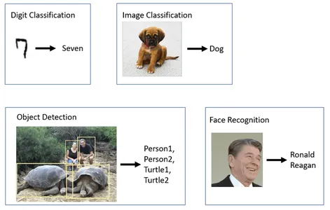
Many computer vision tasks widely use transfer learning, particularly in object detection, where experts fine-tune pre-trained models such as ResNet, VGG, or MobileNet for specific object recognition tasks. Some models like FaceNet and OpenFace employ transfer learning to recognize faces across different lighting conditions, poses, and angles. Pre-trained models are adapted for image classification tasks also. These include medical image analysis, wildlife monitoring, and quality control in manufacturing.

Natural Language Processing (NLP):

There are some transfer learning models like BERT and GPT where these models are finetuned for sentiment analysis. So that they can be able to understand the sentiment of the text in various situations, Google’s Transformer model uses transfer learning to translate text between languages.

Autonomous Vehicles:

The application of transfer learning in autonomous vehicles is a rapidly evolving and critical development area in the automotive industry. There are many segments in this area where transfer learning is used. Some are object detection, object recognition, path planning, behavior prediction, sensor fusion, traffic controls, and many more.

Content Generation:

Content generation is an exciting application of transfer learning. GPT-3 (Generative Pre-trained Transformer 3) has been trained on vast amounts of text data. It can generate creative content in many domains. GPT-3 and other models generate creative content, including art, music, storytelling, and code generation.

Recommendation Systems:

We all know the advantages of recommendation systems. It simply makes our lives a little bit simpler, and yes, we use transfer learning here too. Many online platforms, including Netflix and YouTube, use transfer learning to recommend movies and videos based on user preferences.

Learn More: Understanding Transfer Learning for Deep Learning

Enhancing Generative Models

Generative models are one of the most exciting and revolutionary concepts in the fast-evolving field of artificial intelligence. In many ways, transfer learning can improve the functionality and performance of generative ai models like GANs (Generative Adversarial Networks) or VAEs (Variational Autoencoders). One of the primary benefits of transfer learning is that it allows models to use acquired knowledge on different related tasks. We know that generative models require extensive training. To achieve better results, training it on large datasets is essential, a practice strongly endorsed by transfer learning. Instead of starting from scratch, models can initiate activity with pre-existing knowledge.

In the case of GANs or VAEs, experts can pre-train the discriminator or encoder-decoder parts of the model on a broader dataset or domain. This can speed up the training process. Generative models usually need vast amounts of domain-specific data to generate high-quality content. Transfer learning can resolve this issue as it requires only smaller datasets. It also facilitates the continual learning and adaptation of generative models.

Transfer learning has already found practical applications in improving generative ai models. It has been used to adapt text-based models like GPT-3 to generate images and write code. In the case of GANs, transfer learning can help create hyper-realistic images. As generative ai keeps getting better, transfer learning will be super important in helping it do even more excellent stuff.

MobileNet V2

Google created MobileNetV2, a robust pre-trained neural network architecture widely used in computer vision and deep learning applications. They initially intended this model to handle and analyze images quickly, aiming to achieve cutting-edge performance on a variety of tasks. It is now a well-liked option for many computer vision tasks. MobileNetV2 is specifically designed to be lightweight and efficient. It takes a relatively small number of parameters and achieves highly accurate, impressive results.

Despite its efficiency, MobileNetV2 maintains high accuracy in various computer vision tasks. MobileNetV2 introduces the concept of inverted residuals. Unlike traditional residuals, where the output of a layer is added to its input, inverted residuals use a shortcut connection to add the information to the production. It makes the model deeper and more efficient.

Inverted residuals use a shortcut connection to add the information to the production, unlike traditional residuals where the output of a layer is added to its input. You can take this pre-trained MobileNetV2 model and finetune it for specific applications. Thus, it saves lots of time as well as computational resources, leading to the reduction of computational cost. Because of its effectiveness and efficiency, MobileNetV2 is widely used in industry and research. TensorFlow Hub offers easy access to pre-trained MobileNetV2 models. It makes it simple to integrate the model into Tensorflow-based-projects.

Rock-Paper-Scissors Classification

Let’s start building a machine-learning model for the rock-paper-scissors classification task. We will use the transfer learning technique to implement. For that, we use the MobileNet V2 pre-trained model.

Rock-Paper-Scissors Dataset

The ‘Rock Paper Scissors’ dataset is a collection of 2,892 images. It consists of diverse hands in all three different poses. These are,

1. Rock: The clenched fist.
2. Paper: The open palm.
3. Scissors: The two extended fingers forming a V.

The images include hands from people of different races, ages, and genders. All the pictures have the same plain white background. This diversity makes it a valuable resource for machine learning and computer vision applications. This helps to prevent both overfitting and underfitting.

Loading and Exploring the Dataset

Let’s start by importing the basic required libraries. This project requires tensorflow, tensorflow hub, tensorflow datasets for dataset, matplotlib for visualization, numpy, and os.

import tensorflow as tf
import tensorflow_hub as hub
import tensorflow_datasets as tfds
import matplotlib.pylab as plt
import numpy as np
import os

Using tensorflow datasets, load the “Rock Paper Scissors” dataset. Here, we are providing four parameters to it. We have to mention the name of the dataset that we need to load. Here it is rock_paper_scissors. To request information about the dataset, set with_info to True. Next, to load the dataset in the supervised format, set as_supervised to True.

And at last, define the splits that we want to load. Here, we need to train and test partitions. Load datasets and info to corresponding variables.

datasets, info = tfds.load(
    name="rock_paper_scissors",  # Specify the name of the dataset you want to load.
    with_info=True,              # To request information about the dataset
    as_supervised=True,          # Load the dataset in a supervised format.
    split=('train', 'test')     # Define the splits you want to load.
)

Print Info

Now print the info. It will publish all the details of the dataset. It’s name, version, description, original dataset resource, features, total number of images, split numbers, author, and many more details.

info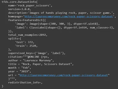

Now, print some sample images from the training dataset.

train, info_train = tfds.load(name="rock_paper_scissors", with_info=True, split="train")
tfds.show_examples(info_train,train)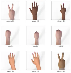

We first load the “Rock Paper Scissors” dataset with the kids. Load () function, specifying the training and testing splits separately. Then, we concatenate the training and testing datasets using the .concatenate() method. Finally, we shuffle the combined dataset using the .shuffle() method with a buffer size 3000. Now, you have a single dataset variable that combines training and testing data.

dataset=datasets(0).concatenate(datasets(1))
dataset=dataset.shuffle(3000)

We must split the entire dataset into training, testing, and validation datasets using skip() and take() methods. We use the first 600 samples of the dataset for validation. Then, we create a temporary dataset by excluding the initial 600 images. In this temporary dataset, we select the first 400 photos for testing. Again, in the training dataset, it takes all the pictures of the temporary dataset after skipping the first 400 images.

Here’s a summary of how data is split:

• rsp_val: 600 examples for validation.
• rsp_test: 400 samples for testing.
• rsp_train: The remaining examples for training.

rsp_val=dataset.take(600)
rsp_test_temp=dataset.skip(600)
rsp_test=rsp_test_temp.take(400)
rsp_train=rsp_test_temp.skip(400)

So, let’s see how many images are in the training dataset.

len(list(rsp_train))

#1892
#It has 1892 images in total

Data Preprocessing

Now, let’s perform some preprocessing for our dataset. For that, we will define a function scale. We will pass the image and its corresponding label as arguments to it. Using the cast method, we will convert the data type of the image to float32. Then, in the next step, we have to normalize the image’s pixel values. It scales the image’s pixel values to the range (0, 1). Image resizing is a common preprocessing step to ensure that all input images have the exact dimensions, often required when training deep learning models. So, we will return the images of size (224,224). For the labels, we will perform onehot encoding. The label will be converted into a one-hot encoded vector if you have three classes (Rock, Paper, Scissors). This vector is being returned.

For example, if the label is 1 (Paper), it will be transformed into (0, 1, 0). Here, each element corresponds to a class. The “1” is placed in the position corresponding to that particular class (Paper). Similarly, for rock labels, the vector will be (1, 0, 0), and for scissors, it will be (0, 0, 1).

Code

def scale(image, label):
  image = tf.cast(image, tf.float32)
  image /= 255.0

  return tf.image.resize(image,(224,224)), tf.one_hot(label, 3)

Now, define a function to create batched and preprocessed datasets for training, testing, and validation. Apply the predefined scale function to all three datasets. Define the batch size as 64 and pass it as an argument. This is common in deep learning, where models are often trained on batches of data rather than individual examples. We need to shuffle the train dataset to avoid overfitting. Finally, return all the three scaled datasets.

def get_dataset(batch_size=64):
  train_dataset_scaled = rsp_train.map(scale).shuffle(1900).batch(batch_size)
  test_dataset_scaled =  rsp_test.map(scale).batch(batch_size)
  val_dataset_scaled =  rsp_val.map(scale).batch(batch_size)
  return train_dataset_scaled, test_dataset_scaled, val_dataset_scaled

Load the three datasets individually using the get_dataset function. Then, cache train and validation datasets. Caching is a valuable technique to improve data loading performance, especially when you have enough memory to store the datasets. Caching means the data is loaded into memory and kept there for faster access during training and validation steps. This can speed up training, especially if your training process involves multiple epochs, because it avoids repeatedly loading the same data from storage.

train_dataset, test_dataset, val_dataset = get_dataset()
train_dataset.cache()
val_dataset.cache()

Loading Pre-Trained Model

Using Tensorflow Hub, load a pre-trained MobileNet V2 feature extractor. And configure it as a layer in a Keras model. This MobileNet model is trained on a large dataset and can be used to extract features from images. Now, create a keras layer using the MobileNet V2 feature extractor. Here, specify the input_shape as (224, 224, 3). This indicates that the model expects input images with dimensions 224×224 pixels and three color channels (RGB). Set the trainable attribute of this layer to False. Doing this indicates that you do not want to finetune the pre-trained MobileNet V2 model during your training process. But you can add your custom layers on top of it.

feature_extractor = "https://tfhub.dev/google/tf2-preview/mobilenet_v2/feature_vector/4"
feature_extractor_layer = hub.KerasLayer(feature_extractor, input_shape=(224,224,3))
feature_extractor_layer.trainable = False

Building Model

It’s time to build the TensorFlow Keras Sequential model by adding layers to the MobileNet V2 feature extractor layer. To the feature_extractor_layer, we will add a dropout layer. We will set a dropout rate of 0.5 here. This regularisation method is what we do to avoid overfitting. During training, if the dropout rate is set to 0.5, the model will drop an average of 50% of the units. Afterward, we add a dense layer with three output units, and in this step, we use the ‘softmax’ activation function. ‘Softmax’ is a widely used activation function for solving multi-class classification problems. It computes the probability distribution over each input image’s classes (Rock, Paper, Scissors). Then, print the summary of the model.

model = tf.keras.Sequential((
  feature_extractor_layer,
  tf.keras.layers.Dropout(0.5),
  tf.keras.layers.Dense(3,activation='softmax')
))

model.summary()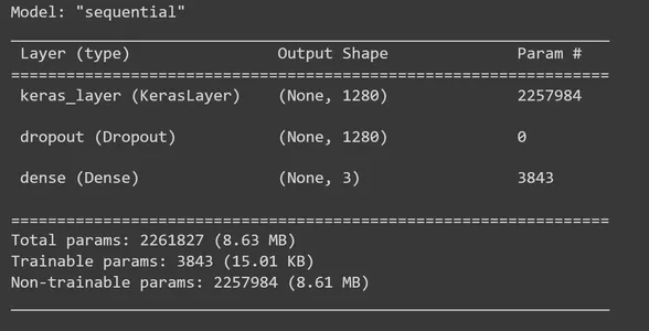

It’s time to compile our model. For this, we use the Adam optimizer and C.ategoricalCrossentropy loss function. The from_logits=True argument indicates that your model’s output produces raw logits (unnormalized scores) instead of probability distributions. To monitor during the training, we use accuracy metrics.

model.compile(
  optimizer=tf.keras.optimizers.Adam(),
  loss=tf.keras.losses.CategoricalCrossentropy(from_logits=True),
  metrics=('acc'))

Functions called callbacks can be executed at different stages of training, including the end of each batch or epoch. In this context, we define a custom callback in TensorFlow Keras with the purpose of gathering and recording loss and accuracy values at the batch level during training.

class CollectBatchStats(tf.keras.callbacks.Callback):
  def __init__(self):
    self.batch_losses = ()
    self.batch_acc = ()

  def on_train_batch_end(self, batch, logs=None):
    self.batch_losses.append(logs('loss'))
    self.batch_acc.append(logs('acc'))
    self.model.reset_metrics()

Now, create an object of the created class. Then, train the model using the fit_generator method. To do this, we need to provide the necessary parameters. We need a training dataset mentioning the number of epochs it needs to train, the validation dataset, and set callbacks.

batch_stats_callback = CollectBatchStats()

history = model.fit_generator(train_dataset, epochs=5, validation_data=val_dataset,
                              callbacks = (batch_stats_callback))

Visualizations

Using matplotlib, plot the training loss over training steps using the data collected by the CollectBatchStats callback. We can observe how the loss is optimized in the field as the training progresses.

plt.figure()
plt.ylabel("Loss")
plt.xlabel("Training Steps")
plt.ylim((0,2))
plt.plot(batch_stats_callback.batch_losses)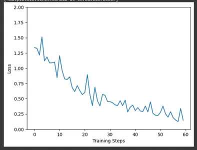

Similarly, plot accuracy over training steps. Here also, we can observe the increase in accuracy as the training progresses.

plt.figure()
plt.ylabel("Accuracy")
plt.xlabel("Training Steps")
plt.ylim((0,1))
plt.plot(batch_stats_callback.batch_acc)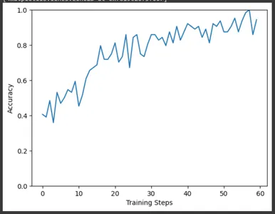

Evaluation and Results

It’s time to evaluate our model using a test dataset. The result variable will contain the evaluation results, including test loss and any other metrics you defined during model compilation. Extract the test loss and test accuracy from the result array and print them. We will get a loss of 0.14 and an accuracy of around 96% for our model.

result=model.evaluate(test_dataset)
test_loss = result(0)  # Test loss
test_accuracy = result(1)  # Test accuracy
print(f"Test Loss: {test_loss}")
print(f"Test Accuracy: {test_accuracy}")

#Test Loss: 0.14874716103076935
#Test Accuracy: 0.9674999713897705

Let’s see the prediction for some test images. This loop iterates through the first ten samples in the rsp_test dataset. Apply the scale function to preprocess the image and label. We perform scaling the image and one-hot encoding of the brand. It will print the actual label (converted from a one-hot encoded format) and the predicted label (based on the class with the highest probability in the predictions).

for test_sample in rsp_test.take(10):  
  image, label = test_sample(0), test_sample(1)
  image_scaled, label_arr= scale(test_sample(0), test_sample(1))
  image_scaled = np.expand_dims(image_scaled, axis=0)   

  img = tf.keras.preprocessing.image.img_to_array(image)                    
  pred=model.predict(image_scaled)
  print(pred)
  plt.figure()
  plt.imshow(image)
  plt.show()
  print("Actual Label: %s" % info.features("label").names(label.numpy()))
  print("Predicted Label: %s" % info.features("label").names(np.argmax(pred)))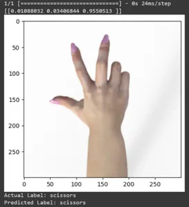

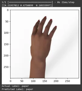
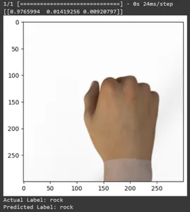
Let’s print predictions of all test images. It will generate forecasts for the entire test dataset using your trained TensorFlow Keras model and then extract the class labels (class indices) with the highest probability for each prediction.

np.argmax(model.predict(test_dataset),axis=1)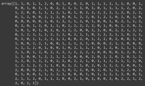

Print confusion matrix for the model’s predictions. The confusion matrix provides a detailed breakdown of how the model’s predictions align with the labels. It’s a valuable tool for assessing the performance of a classification model. It gives each class true positives, true negatives, and false positives.

for f0,f1 in rsp_test.map(scale).batch(400):
  y=np.argmax(f1, axis=1)
  y_pred=np.argmax(model.predict(f0),axis=1)
  print(tf.math.confusion_matrix(labels=y, predictions=y_pred, num_classes=3))
 
#Output 
tf.Tensor(
((142   3   0)
 (  1 131   1)
 (  0   1 121)), shape=(3, 3), dtype=int32)
 
 

Saving and Loading the Trained Model

Save the trained model. So that when you need to use the model, you don’t have to teach everything from scratch. You have to load the model and use it for prediction.

model.save('./path/', save_format="tf")

Let’s check the model by loading it.

loaded_model = tf.keras.models.load_model('path')

Similarly, like we had done earlier, let’s test the model with some sample images in the test dataset.

for test_sample in rsp_test.take(10):  
  image, label = test_sample(0), test_sample(1)
  image_scaled, label_arr= scale(test_sample(0), test_sample(1))
  image_scaled = np.expand_dims(image_scaled, axis=0)   

  img = tf.keras.preprocessing.image.img_to_array(image)                    
  pred=loaded_model.predict(image_scaled)
  print(pred)
  plt.figure()
  plt.imshow(image)
  plt.show()
  print("Actual Label: %s" % info.features("label").names(label.numpy()))
  print("Predicted Label: %s" % info.features("label").names(np.argmax(pred)))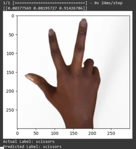

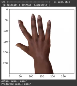
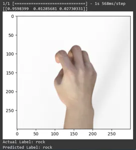
Conclusion

In this article, we have applied transfer learning for the Rock-Paper-Scissors classification task. We have used a pre-trained Mobilenet V2 model for this task. Our model is working successfully with an accuracy of around 96%. In the predictions images, we can see how well our model is predicting. The last three shots show how perfect it is, even if the hand pose is imperfect. To represent “scissors,” open three fingers instead of using a two-finger configuration. For “Rock,” don’t form a fully clenched fist. But still, our model can understand the corresponding class and predict perfectly.

Key Takeaways

• Transfer learning is all about transferring knowledge. The knowledge gained in the previous task is used in learning a new job.
• Transfer learning has the potential to revolutionize the machine learning field. It provides several benefits, including accelerated learning and improved performance.
• Transfer learning promotes continuous learning, where models can change over time to deal with new information, tasks, or the environment.
• It is a flexible and effective method that raises the effectiveness and efficiency of machine learning models.
• In this article, we have learned all about transfer learning, its benefits, and applications. We also implemented using a pre-trained model on a new dataset to perform the rock-paper-scissors classification task.

Frequently Asked Questions (FAQs)

The media shown in this article is not owned by Analytics Vidhya and is used at the Author’s discretion.

Related