Introduction to HNSW: Hierarchical Navigable Small World

Introduction

ai innovation is happening at breakneck speed. One of the frontiers of this innovation is the vector search engines. What are these search engines, you ask? In simple terms, they help in training large language models (LLMs) by going through large datasets and picking out what’s relevant. Now, there are many different ways in which this indexing is done in vector databases. Among them, Hierarchical Navigable Small World (HNSW) stands out for being performant and scalable. All the major vector stores provide HNSW as an indexing method. It is fast, efficient, robust, and reliable. So, in this article, we will break down the inner workings of HNSW and learn what makes it so fast.

Learning Objectives

• Understand what embeddings and vector databases are.
• Get familiar with the different ways of indexing in vector databases.
• Learn what HNSW is and how it works.
• Understand HNSWlib, a header-only HNSW implementation.

This article was published as a part of the Data Science Blogathon.

What are Embeddings?

Embeddings are vector representations of data (text, image) in a high-dimensional vector space.

Two semantically related data will be in proximity in the vector space, while dissimilar data will be far away. In other words, the word embeddings for Messi and football will be close together in the embedding space, while the word embeddings for football and Joe Biden will be far apart in the embedding space.

The length of vectors can range from a few hundred to thousands or more. This makes it difficult to store, query, and search. But every Retrieval Augmented Generation (RAG) based application requires high-speed search and querying of data embeddings. This is where Vector Databases come into the picture.

What are Vector Databases?

Just as traditional databases aim to store structured and unstructured data, vector databases store, search, and query high-dimensional vector embeddings. They provide user-friendly interfaces to interact with embeddings and their associated data. Vector databases are not fundamentally different from traditional databases. Vector databases use traditional databases to store serialized embeddings. For example, Chroma uses SQLite as in-memory storage, and Pgvector uses the Postgres database to store embeddings and their associated metadata. The thing that separates a traditional database from a vector database is the underlying indexing algorithm.

Indexing in Vector Databases

Indexing refers to the process of organizing high-dimensional vectors in a way that provides efficient querying of nearest-neighbor vectors.

This is the most crucial part of building any vector database. These indexes enable fast and efficient querying of high-dimensional embeddings. There are multiple indexing methods to create vector indices, such as:

• Linear search Algorithm (Flat Indexing): This is a linear search algorithm, which means it will compare the query vector with every other vector stored in the database. This is the simplest method out there and works well with small datasets.
• Cluster-based algorithm (IVF): Inverted File is a cluster-based indexing technique. It uses k-means clustering to cluster all the vectors. When a query vector is provided, it calculates the distance between the query vector and the centroids of each cluster. And starts searching for the nearest neighbors in the cluster with the centroid closest to the query vector. This significantly reduces query time.
• Quantization (Scalar and Product Quantization): The quantization technique involves reducing the memory footprint of large embeddings by reducing their precision.
• Graph-based (HNSW): The most common indexing method. It uses hierarchical graph architecture to index vectors. And this is what we are going to explore.

Understanding HNSW

Large language models (LLMs) are becoming increasingly popular, and many organizations want to implement them in their product stacks. However, there is a challenge to doing this: LLMs have a limited context window. A context window is the number of tokens an ai model can ingest. For example, the GPT 3.5 turbo has a context length of 4096. This is where vector search databases shine. Instead of throwing the entire book into the context of LLM, we find the most relevant parts and feed them to the LLM to get precise outcomes.

Now, amongst all the different ways of indexing in vector databases discussed above, HNSW is the most robust and scalable. This makes it the most widely used indexing method as well. HNSW is formed by combining two algorithms: skip list and navigable small world. To understand HNSW, we need to know these algorithms. So, let’s dive in.

Skip List

As the name suggests, the Skip list is based on the linked list data structure, or we can say it is an extension of the linked list data structure. It was invented by David Pugh in 1990 as a faster alternative to linked lists.

Why do we even need a skip list? A linked list has an O(n) search time complexity. This may not be ideal for real-world use cases where speed of execution is paramount. So, this is why we may need a more efficient linked-list algorithm.

The skip lists have an expected time complexity of O(log n). It performs much better at random access than linked lists. As it has a layered structure with multiple nodes at each layer, the worst-case space complexity is O(n log n), where n is the number of nodes at the bottom-most level.

How Does Skip List Work?

A Skip list maintains a layered linked architecture where the top layer has the longest links between elements. This reduces exponentially as we move down the layers.

In the above picture, the bottom-most layer is a complete linked list. As we move up, the number of nodes reduces by half in each layer. The structure is called skip lists, as the higher layers let you skip nodes while traversing.

Consider the following example.

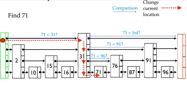
When searching for k:

• if k = target element
• if k >= move right
• if k < move down

We start from the top left corner and move right until we find k or a number less than k. We descend to the layer below and continue the process until we reach k. The search complexity is O(log n) as we skip half the items at each level.

While random access is faster, insertion and deletion are slower as they add additional overhead for updating and deleting on multiple layers.

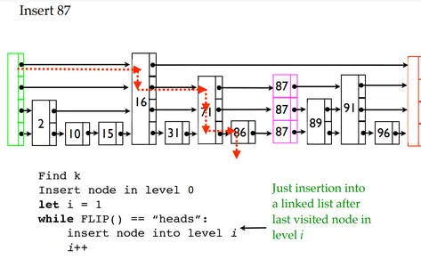
While insertion, we start from the bottom list and add the node at the appropriate position. As skip lists maintain a hierarchical structure, we need to determine if the node appears at a higher level. The process is random, like a coin toss. The probability of a node appearing in its immediate upper layer is 0.5. In an ideal skip list, the number of nodes on layer-1 will be ~n/2, and in layer-2 ~n/4, where n is the number of nodes on the bottom-most layer or the complete linked list.

Consider the following example.

We find the ideal place for insertion and insert the node at the bottom level. We then decide if the node appears on the upper level based on a random binary outcome (heads or tail). In a perfect skip list, we get a balanced distribution of nodes in each level.

Deletion happens similarly. Find the target number and delete the node. If the element is there on a higher layer, delete it and update the linked list.

Navigable Small World (NSW)

Navigable Small World is a graph-based algorithm for finding approximate nearest neighbors. The data points in a graph are called nodes. Each node is linked to a fixed set of connections that are close to each other.

This is a greedy algorithm. It starts at a pre-defined point in the graph and selects nodes closer to the target node. The distance between the nodes can be measured by Euclidean or Cosine similarity. This process is repeated until it reaches the nearest neighbors of the target node.

The Navigable Small World algorithm is very efficient and easily deployable. It works well for datasets ranging from a few hundred to thousands. After that, it tends to perform worse. It suffers from pre-mature termination when it can not find a better neighbor than the current one, as it uses only local information to find the nearest neighbor.

During insertion, we traverse the graph to find the nearest neighbors and connect them to the node x.

As in vector databases, we need to deal with several millions of embedding data. Hence, we need a better algorithm that scales well and offers better searchability. While NSW performs well enough for small datasets, we need an even better algorithm to handle 100s of millions or billions of data points. This is where HNSW comes into the picture.

Hierarchical Navigable Small World (HNSW)

HNSW extends NSW by incorporating the hierarchical architecture of Skip Lists. This removed the scalability bottleneck of NSW. Like Skip Lists, HNSW creates the multi-layer structure of NSWs instead of linked lists. Like Skip Lists, the topmost layer will have fewer data points with the longest connections. The number of elements increases as we move down the hierarchy. At the bottom-most level, we have all the data points. Like skip lists, the probability of the existence of an element exponentially decreases as we move up in the hierarchy.

But how do we search in HNSW?

Searching in HNSW

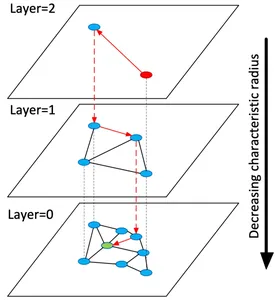
Now recall both the skip list and NSW. In the skip list, we start at the uppermost layer, and in NSW, we start at a pre-defined point. In HNSW, we start from a pre-defined point at the uppermost layer of the hierarchy and greedily traverse the graph to find the closest element to the target data point in that layer. Once we reach the nearest node, we descend to the layer below and repeat the process until “K” nearest neighbors of the target node are found. See below picture

Insertion and Deletion in HNSW

Insertion in HNSW follows the same principle as that of Skip lists. We traverse the layers, finding the nearest neighbors of the element. Then, we move down and repeat the same process until we find all the nearest neighbors on the bottom layer.

The next task is to determine the bi-directional links to the inserted element. It is usually determined by a predefined parameter m. We connect the m number of nearest neighbors to the inserted node. This is one of the ways to determine connections to an inserted node. Other heuristics can also be used. For instance, instead of only connecting to the nearest neighbor nodes of the same region, we also connect the inserted node to the closest node of the nearest region to form a better-connected graph.

As with the skip lists, the probability of a node appearing in the higher layers is decided randomly. The function for it is floor(-ln(rand(0, 1))), where rand(0, 1) is a random number sampled from a uniform distribution between (0, 1).

Deletion follows a similar approach. We start with the top layer and delete the target as it appears till the bottom layer.

Complexities in HNSW

The time complexities of searching, insertion, and deleting in HNSW depend on multiple factors, including the height of the architecture, the number of neighboring nodes per node, and the distance metric. But on average, searching, insertion, and deletion have O(log n) time complexity. The construction of the HNSW can be expensive. We need to insert n number of nodes with O(log n) complexity. So, the overall time complexity of graph construction will be O(n log n).

Vector databases are built to handle hundreds of millions of embeddings. Indexing such an amount of data requires a highly efficient, robust, and scalable algorithm. HNSW ticks all the boxes.

Cons of HNSW

Although the searching, insertion, and deletion are faster in HNSW, there are a few trade-offs you need to know before going with HNSW. Here are a few things to keep in mind before implementing HNSW.

• Higher Memory footprint: HNSW maintains a hierarchical structure of embeddings, which significantly increases memory consumption compared to algorithms like NSW. This can be problematic for resource-constraint devices.
• Parameter Tuning: HNSW has different tunable parameters. Careful parameter tuning is needed to improve performance.
• Difficulty: Implementing HNSW from scratch can get tricky. Most vector databases use trusted pre-built solutions such as FAISS or HNSWlib.

HNSWlib is a header-only C++ implementation of the HNSW algorithm with Python bindings. It was written by the author of the HNSW paper, Yury Malkov. This is a bare-bone implementation of the algorithm.

So, let’s get into it.

You can install HNSWlib with any Python package manager.

pip install hnswlib

Declare and Initialize HNSW index.

import hnswlib
import numpy as np
import pickle

dim = 16
num_elements = 100

hnsw_index = hnswlib.Index(space="l2", dim = dim) #declare Index
hnsw_index.init_index(max_elements = num_elements, ef_construction = 200, M = 16)

• The space parameter is the distance metric that will be used to calculate the distance between nodes. Python implementation supports squared L2, Cosine, and dot-product.
• The dim parameter is the dimension of embedding vectors
• The init_index method initializes the index.
• ef_construction defines the construction time/accuracy trade-off.
• M is the number of bi-directional links created during the insertion of a node.

Now that we created the indexes let’s add a few vectors.

data1 = np.float32(np.random.random((num_elements, dim)))
ids1 = np.arange(num_elements)
data2 = np.float32(np.random.random((100, dim)))
ids2 = np.arange(100)
data3 = np.float32(np.random.random((100, dim)))
ids3 = np.arange(100)

hnsw_index.add_items(data1, ids1)
hnsw_index.add_items(data2, ids2)

hnsw_index.set_ef(50) #set query time speed/accuracy trade-off
hnsw_index.set_num_threads(4) #sets number of threads during batch construction

Now, let’s see how we can query k’s approximate nearest neighbor.

labels, distances = p.knn_query(data, k = 1)

Serialize the index object using pickle.

p_cp = pickle.loads(pickle.dumps(hnsw_index))

Deleting elements.

for id in ids2:
    hnsw_index.mark_deleted(id)

This will free up the last 100 elements from the index. If you wish, you can also reuse the memory of deleted elements.

hnsw_index.add_items(data3, labels3, replace_deleted=True)

Conclusion

The HNSW is one of the most crucial algorithms right now for the development of vector retrieval methods. It is the primary indexing algorithm used in all major vector databases. Hope you’ve understood the workings of HNSW through this article. As ai evolves, we will see the development of larger and more complex learning models, causing a rise in the need for using HNSW and increasing its applications and importance.

Key Takeaways

• Vector databases are purpose-built data stores for storing high-dimensional vector embeddings.
• Indexing of embeddings allows vector stores to handle querying, insertion, and deletion of embeddings.
• There are different ways of indexing vectors, such as IVF, Annoy, Quantization, and HNSW.
• HNSW is a combination of two algorithms. Skip lists and a Navigable Small World (NSW).

Frequently Asked Questions

The media shown in this article is not owned by Analytics Vidhya and is used at the Author’s discretion.

Related