 NEWSLETTER
For my graph, I'm using a historical Olympic dataset from Olympedia.org that Joseph Cheng shared on Kaggle licensed under a public domain license.
It contains results from the Olympic Games from Athens 1896 to Beijing 2022, from event to athlete level. After exploratory data analysis (EDA), I transformed it into a dataset detailing the number of female athletes in each sport/event per year. My idea of the bubble chart is to show which sports have a 50/50 ratio of female to male athletes and how this has evolved over time.
My graph data consists of two different data sets, one for each year: 2020 and nineteen ninety sixFor each data set, I have calculated the total sum of athletes who participated in each event. (sum_athlete) and how much does that sum represent compared to the total number of athletes (men + women) (difference)See a screenshot of the data below:
This is my approach to visualizing it:
- Size proportion. Using bubble radius to compare the number of athletes per sport. Larger bubbles represent highly competitive events, such as track and field.
- Multivariate interpretationUse colors to represent female representation. Light green bubbles will represent events with a 50/50 split, such as hockey.
Here's my starting point (using the code and approach mentioned above):
Some easy solutions: increase the size of the figure and change the labels to empty if the size does not exceed 250 to avoid having words outside the bubbles.
fig, ax = plt.subplots(figsize=(12,8),subplot_kw=dict(aspect="equal"))#Labels edited directly in dataset
Well, at least it's readable now. But why? Athletics pink and Boxing blue? Let's add a legend to illustrate the relationship between colors and female representation.
Because it is not a normal bar graph, plt.legend() It doesn't work here.
With matplotlib's Bbox annotation we can create rectangles (or circles) to show the meaning of each color. We can also do the same to show a bubble scale.
import matplotlib.pyplot as plt
from matplotlib.offsetbox import (AnnotationBbox, DrawingArea,
TextArea,HPacker)
from matplotlib.patches import Circle,Rectangle# This is an example for one section of the legend
# Define where the annotation (legend) will be
xy = (50, 128)
# Create your colored rectangle or circle
da = DrawingArea(20, 20, 0, 0)
p = Rectangle((10 ,10),10,10,color="#fc8d62ff")
da.add_artist(p)
# Add text
text = TextArea("20%", textprops=dict(color="#fc8d62ff", size=14,fontweight='bold'))
# Combine rectangle and text
vbox = HPacker(children=(da, text), align="top", pad=0, sep=3)
# Annotate both in a box (change alpha if you want to see the box)
ab = AnnotationBbox(vbox, xy,
xybox=(1.005, xy(1)),
xycoords='data',
boxcoords=("axes fraction", "data"),
box_alignment=(0.2, 0.5),
bboxprops=dict(alpha=0)
)
#Add to your bubble chart
ax.add_artist(ab)
I also added a caption and text description below the graph simply by using plt.text()
Simple and easy to use chart interpretations:
- Most bubbles are light green → green means 50% women → most Olympic competitions have an even 50/50 split between women and men (yay)
- Only one sport (baseball), in dark green, has no female participation.
- 3 sports have only female participation but the number of athletes is quite low.
- The biggest sports in terms of number of athletes (swimming, track and field and gymnastics) are very close to having a 50/50 split.


