How to Optimize Data Warehouse with STAR Schema?

Introduction

The STAR schema is an efficient database design used in data warehousing and business intelligence. It organizes data into a central fact table linked to surrounding dimension tables. This star-like structure simplifies complex queries, enhances performance, and is ideal for large datasets requiring fast retrieval and simplified joins.

A major advantage of the STAR schema is its ability to minimize the number of query joins, improving readability and performance, especially for data aggregation and reporting. Its straightforward design supports rapid data summarization, which is essential for generating business insights.

The STAR schema also offers scalability, allowing new dimension tables to be added without disrupting the existing structure. This supports ongoing growth and adaptability. Separating fact and dimension tables minimizes data redundancy and maintains consistency.

In this blog, we’ll explore the STAR schema, demonstrate its setup for optimal query performance with simulated data, and compare it with the Snowflake schema, offering a streamlined approach to data management and analysis.

Learning objectives

• Understand the key elements of the STAR schema.
• Learn how to design a STAR schema and understand its advantages in improving query performance.
• Explore how a STAR schema simplifies analytical queries.
• Learn how the STAR schema facilitates data aggregation and reporting.
• Understand how the STAR schema compares with the Snowflake schema and how to choose the right one.

This article was published as a part of the Data Science Blogathon.

What is a STAR Schema?

The STAR schema is a database schema consisting of a central fact table surrounded by dimension tables. Fact tables store measurable, quantitative data, such as sales transactions and customer orders. In contrast, dimension tables store descriptive attributes, such as customer details, product categories, and time information.

A STAR has a structure that resembles a star and is created by connecting the fact and dimension tables using foreign keys. This design is highly optimized for read-heavy operations, especially in reporting and analytical environments.

Key Components of a STAR Schema:

• Fact Table: The fact table stores transactional data. In our example of customer orders, this table would keep track of every order placed by customers.
• Dimension Tables: Dimension tables are supplementary tables with descriptive information about the customers, products, and dates of the entities involved in the transactions.

This structure enables fast querying by simplifying the joins between tables and reducing complexity when extracting insights from data.

Also read: A Brief Introduction to the Concept of Data Warehouse

Example: Customer Orders

To illustrate how the STAR schema works, we’ll generate a simulated dataset representing customer orders in an online store. This data will populate our fact and dimension tables.

1. Customer Data (Dimension Table)

We’ll create a simulated customer dataset, including key information such as their ID, name, location, and membership type. The Customer Data dimension table details each customer and allows us to link orders to specific customers to analyze customer behavior, preferences, and demographic trends.

• customer_id: A unique identifier for each customer. This ID will be used as a foreign key in the Orders fact table to link each transaction to the customer who placed the order.
• first_name: The customer’s first name. This is part of the customer’s identifying information.
• last_name: The customer’s last name. Together with the first name, this provides full identification of the customer.
• Location: This field contains the customer’s geographic location (e.g., country or region). It can be used to analyze customer orders based on geography.
• membership_level: Indicates whether the customer has a Standard or Premium membership. This allows for customer behavior analysis by membership type (e.g., do premium customers spend more?).

import pandas as pd
import numpy as np

def generate_customer_data(n_customers=1000):
    np.random.seed(42)
    customer_ids = np.arange(1, n_customers + 1)
    first_names = np.random.choice(('Thato', 'Jane', 'Alice', 'Bob'), size=n_customers)
    last_names = np.random.choice(('Smith', 'Mkhize', 'Brown', 'Johnson'), size=n_customers)
    locations = np.random.choice(('South Africa', 'Canada', 'UK', 'Germany'), size=n_customers)
    membership_levels = np.random.choice(('Standard', 'Premium'), size=n_customers)
    customers = pd.DataFrame({
        'customer_id': customer_ids,
        'first_name': first_names,
        'last_name': last_names,
        'location': locations,
        'membership_level': membership_levels
    })
    return customers

customers_df = generate_customer_data()
customers_df.head()

Output:

Also read: A Complete Guide to Data Warehousing in 2024

2. Product Data (Dimension Table)

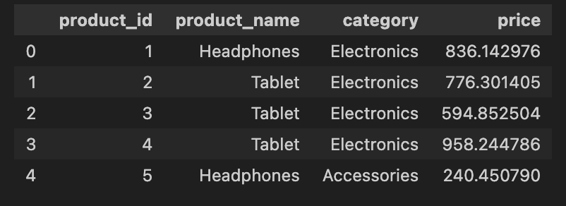
Next, we’ll create a dataset for products that are available for purchase. This data will include fields like product ID, product name, category, and price.

• product_id: A unique identifier for each product. This ID will be used as a foreign key in the Orders fact table to connect the product purchased in each transaction.
• product_name: The name of the product (e.g., Laptop, Phone, Headphones). This field provides descriptive information about the product for analysis and reporting.
• Category: The product category (e.g., Electronics, Accessories). Categories help group and analyze sales performance by product type.
• Price: The price of the product. The product’s unit price will be used to calculate the total price in the fact table (when multiplied by the quantity).

def generate_product_data(n_products=500):
    product_ids = np.arange(1, n_products + 1)
    product_names = np.random.choice(('Laptop', 'Phone', 'Tablet', 'Headphones'), size=n_products)
    categories = np.random.choice(('Electronics', 'Accessories'), size=n_products)
    prices = np.random.uniform(50, 1000, size=n_products)
    products = pd.DataFrame({
        'product_id': product_ids,
        'product_name': product_names,
        'category': categories,
        'price': prices
    })
    return products

products_df = generate_product_data()
products_df.head()

Output:

3. Dates Data (Dimension Table)

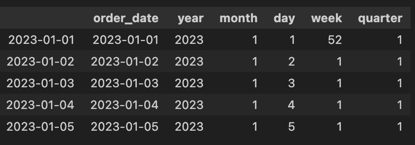
The dates dimension table is crucial for time-based analysis in any data warehousing or business intelligence scenario. It allows you to aggregate and analyze data based on specific periods such as year, month, day, or quarter. This table will reference the transaction’s time, allowing us to link each order to its corresponding date.

• order_date: The actual date of the order, which the Orders fact table will reference.
• year: The year the order was placed.
• month: The month of the order (from 1 to 12).
• day: The day of the month.
• week: The week of the year (based on the ISO calendar).
• quarter: The quarter of the year (1 for January-March, 2 for April-June, and so on).

import pandas as pd

def generate_dates_data(start_date="2023-01-01", end_date="2024-02-21"):
    # Create a date range
    date_range = pd.date_range(start=start_date, end=end_date, freq='D')
    
    # Create a DataFrame with date parts
    dates_df = pd.DataFrame({
        'order_date': date_range,
        'year': date_range.year,
        'month': date_range.month,
        'day': date_range.day,
        'week': date_range.isocalendar().week,
        'quarter': date_range.quarter
    })
    
    return dates_df

# Generate the Dates dimension table
dates_df = generate_dates_data()
dates_df.head()

Output:

Also read: What is Data Warehousing?

4. Orders Data (Fact Table)

Finally, we’ll generate the order data that acts as the fact table. This dataset will track customer orders, including the order date, total price, and product information. Each row in the Orders fact table represents a unique order placed by a customer, and it links directly to the relevant dimension tables (Customers, Products, and Dates) through foreign keys. This allows for detailed analysis, such as tracking how much each customer spends, which products are most popular, and how order activity varies over time.

• order_id: A unique identifier for each order. This serves as the primary key for the fact table.
• customer_id: A foreign key that links each order to a customer in the Customers dimension table. This allows for the analysis of orders based on customer attributes like location or membership level.
• product_id: A foreign key that links each order to a product in the Products dimension table. This allows for analysis of product sales, trends, and performance.
• order_date: A foreign key that links each order to a specific date in the Dates dimension table. This field enables time-based analysis, such as sales by month or quarter.
• quantity: The number of units of the product ordered. This is essential for calculating the total price of the order and understanding purchasing patterns.
• total_price: The total price of the order is calculated by multiplying the product price by the quantity ordered. This is the primary metric for analyzing revenue.

def generate_order_data(n_orders=10000):
    order_ids = np.arange(1, n_orders + 1)
    customer_ids = np.random.randint(1, 1000, size=n_orders)
    product_ids = np.random.randint(1, 500, size=n_orders)
    order_dates = pd.date_range('2023-01-01', periods=n_orders, freq='H')
    quantities = np.random.randint(1, 5, size=n_orders)
    total_prices = quantities * np.random.uniform(50, 1000, size=n_orders)
    orders = pd.DataFrame({
        'order_id': order_ids,
        'customer_id': customer_ids,
        'product_id': product_ids,
        'order_date': order_dates,
        'quantity': quantities,
        'total_price': total_prices
    })
    return orders

orders_df = generate_order_data()
orders_df.head()

Output:

Designing the STAR Schema

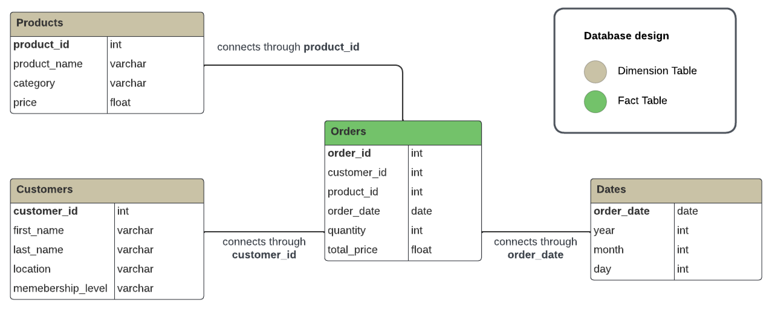
We can now construct the STAR schema using the simulated customer order data. The primary fact table will consist of orders, while the associated dimension tables will encompass customers, products, and dates.

STAR Schema Design:

• Fact Table:
  • orders: contains transactional data, including order_id, customer_id, product_id, order_date, quantity, and total_price.
• Dimension Tables:
  • customers: contains descriptive data about customers, including customer_id, first_name, last_name, location, and membership_level.
  • products: contains product details, including product_id, product_name, category, and price.
  • dates: tracks the dates of each order, including fields like order_date, year, month, and day.

The STAR schema design simplifies queries, as each dimension table directly relates to the fact table, reducing the complexity of SQL joins.

Also read: Understanding the Basics of Data Warehouse and its Structure

Querying the STAR Schema for Business Insights

Now that our schema is in place assume these 4 tables (orders, customers, products, dates) have been created and stored in a SQL database with the same schema as the above dataframes generated for each respective table. With this setup, we can run SQL queries to gain valuable business insights from the data.

Example 1: Total Sales by Product Category

We can easily retrieve total sales by product category using the Orders fact table and the Products dimension table. This query sums the total_price from the Orders table and groups the results by the product category from the Products table:

SELECT
  p.category,
  SUM(o.total_price) AS total_sales
FROM
  orders o
JOIN
  products p
ON
  o.product_id = p.product_id
GROUP BY
  p.category
ORDER BY
  total_sales DESC;

Example 2: Average Order Value by Customer Membership Level

We can join the orders and customers tables to understand how different membership levels affect order value. This query shows whether premium members spend more on average than standard members.

SELECT
  c.membership_level,
  AVG(o.total_price) AS avg_order_value
FROM
  orders o
JOIN
  customers c
ON
  o.customer_id = c.customer_id
GROUP BY
  c.membership_level
ORDER BY
  avg_order_value DESC;

STAR Schema vs Snowflake Schema

The primary difference between the STAR schema and the Snowflake schema is found in the organization of dimension tables, specifically regarding the degree of normalization implemented within those tables. 

1. What is a Snowflake Schema?

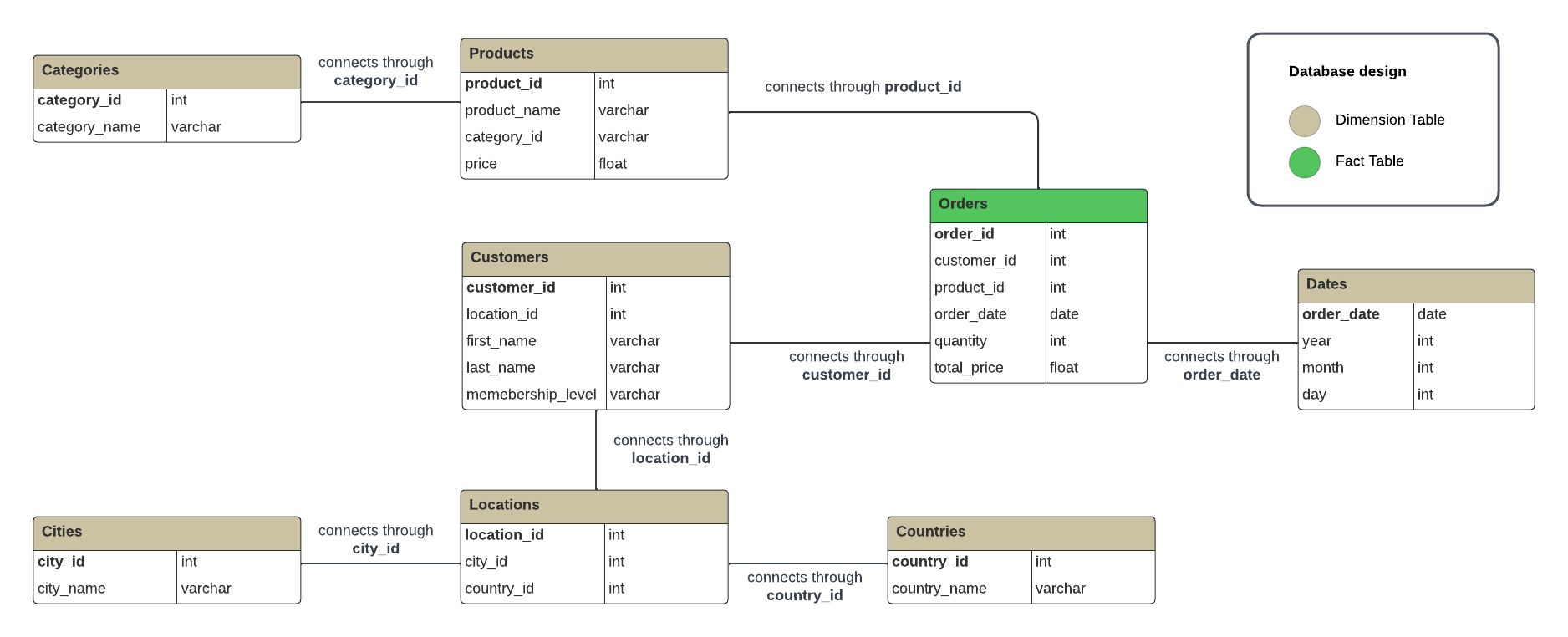
A Snowflake schema is a type of database schema that organizes dimension tables through normalization into several interconnected tables. Unlike the STAR schema, which features denormalized dimension tables, the Snowflake schema further divides dimension tables into sub-dimensions. For instance, a dimension table representing locations may be further segmented into distinct tables for cities and countries. This arrangement leads to a more intricate, hierarchical structure that resembles a snowflake, which is the origin of its name.

Below is a comparison that outlines when to use each schema:

2. The Structure

Here’s the structure:

STAR Schema:

• The dimension tables are denormalized, meaning they are flat and contain all the necessary details. This structure directly links the dimension tables to the central fact table, leading to fewer query joins.
• For instance, in the STAR schema pertaining to our customer order example, the Customer dimension table contains all customer information (e.g., customer_id, first_name, last_name, and location) in a single table.

Snowflake Schema:

• The dimension tables are normalized and broken down into multiple related tables. Each dimension table is split into sub-dimensions based on hierarchy (e.g., breaking down location into city and country tables).
• Example: In a Snowflake schema, the Customers table could be further broken down into a separate Locations table that links customer_id to different hierarchical levels of geographic data, such as City and Country.

3. Query Performance

Here’s the query performance of STAR Schema and Snowflake Schema:

STAR Schema:

• Denormalized dimension tables result in fewer joins, improving query performance for read-heavy operations, especially in analytical queries and reporting.

Snowflake Schema:

• Requires more joins to connect the normalized tables, leading to slower query performance, especially in complex queries.

4. Storage Efficiency

Here is the storage efficiency of STAR Schema and Snowflake Schema:

STAR Schema:

• Since dimension tables are denormalized, there is often some data redundancy, requiring more storage. However, the query simplicity and performance improvements typically outweigh this storage cost.

Snowflake Schema:

• The Snowflake schema reduces redundancy by normalizing dimension tables, making it more storage-efficient. This is beneficial for large-scale datasets where avoiding redundancy is a priority.

5. Scalability

Here’s the scalability of STAR Schema and Snowflake Schema:

STAR Schema:

• The STAR schema’s simple, denormalized structure makes it easier to scale and maintain. Adding new attributes or dimension tables is straightforward and does not require reworking the schema.

Snowflake Schema:

• While the Snowflake schema can handle more complex relationships, it may require more effort to scale and maintain due to the multiple levels of normalization of the dimension tables.

Designing the Snowflake Schema for Customer Orders

Let’s extend the customer orders data example to a Snowflake schema. Instead of storing all customer information in one Customer table, we will break it down to normalize data and reduce redundancy.

Snowflake Schema Structure:

In a Snowflake schema for the same customer order data, we would have the following:

• A Fact Table: Orders table with order_id, customer_id, product_id, order_date, quantity, and total_price.
• Dimension Tables: Instead of keeping denormalized dimension tables, we break them down into further related tables. For instance:
• Customers Table:
  • customer_id, first_name, last_name, location_id, membership_level
• Locations Table:
  • location_id, city_id, country_id
• Cities Table:
• Countries Table:
• Products Table:
  • product_id, product_name, category_id, price
• Categories Table:
  • category_id, category_name

The Orders fact table still contains transactional data, but the customer and product information are normalized across multiple tables (e.g., customer location will link to different levels of geographic data).

Querying the Snowflake Schema Example

To retrieve total sales by product category in a Snowflake schema, you would join several tables to get the final results. Here’s an example SQL query:

SELECT
  c.category_name,
  SUM(o.total_price) AS total_sales
FROM
  orders o
JOIN
  products p
ON
  o.product_id = p.product_id
JOIN
  categories c
ON
  p.category_id = c.category_id
GROUP BY
  c.category_name
ORDER BY
  total_sales DESC;

As you can see, due to the normalized dimension tables, the Snowflake schema requires additional joins compared to the STAR schema. This results in more complex queries but minimizes redundancy in storage.

Conclusion 

In summary, the STAR schema is optimized for fast query performance and simplicity in analytical queries, while the Snowflake schema is designed to reduce redundancy by normalizing dimension tables. The choice between the two depends on the dataset’s specific needs and the organization’s priorities, whether that be query performance or storage efficiency.

In this article, we illustrated constructing a STAR and Snowflake schema utilizing a simulated dataset of customer orders. We fact and dimension tables for customers, products, orders, and dates, demonstrating the essential function of each table in organizing data for effective querying and analysis. This schema allows for the connection of the fact table (orders) to the dimension tables (customers, products, and dates) via foreign keys such as product_id and customer_id, thereby streamlining data retrieval and promoting versatile querying.

We also highlighted key benefits of the STAR schema:

• Simplified Queries: Implementing the STAR schema has illustrated how SQL queries can be made more straightforward, exemplified by our query for total sales categorized by product type.
• Query Performance: The STAR schema design promotes quicker query execution by reducing the number of necessary joins and efficiently aggregating data.
• Scalability and Flexibility: We demonstrated how each dimension table could be expanded with new attributes or rows and how the STAR schema can scale easily as business data grows or requirements change.
• Data Aggregation and Reporting: We demonstrated the ease of performing data aggregation and reporting tasks, such as calculating total sales by product category or monthly trends, thanks to the structure of the STAR schema.

The Snowflake schema reduces data redundancy by normalizing dimension tables, improving storage efficiency but requiring more complex queries. It is ideal for managing hierarchical relationships or optimizing storage space. In contrast, the STAR schema simplifies data management and speeds up query performance, making it better for quick insights and efficient analysis. The choice between the two depends on whether you prioritize query performance or storage efficiency.

Key Takeaways

1. The STAR schema enhances data organization and improves query performance by categorizing transactional data into fact and dimension tables.
2. The schema design supports fast querying, making it easier to derive insights into sales trends, customer behavior, and product performance.
3. The STAR schema is designed for scalability, permitting straightforward expansion as datasets increase. New dimension tables or extra attributes can be added without affecting the current schema, thus ensuring adaptability to changing business requirements.
4. The Snowflake schema minimizes data redundancy by normalizing dimension tables, making it more storage-efficient. However, the need for additional joins can potentially lead to more complex queries.

The media shown in this article are not owned by Analytics Vidhya and is used at the Author’s discretion. 

Frequently Asked Questions