Graphic Neural Networks Part 3: How the Grafsage handle the graphics structure changing

Parts of this series, we analyze the GRAPH convolutionary networks (GCN) and the graphics care networks (GATS). Both architectures work well, but they also have some limitations! A great is that for large graphics, calculate the node representations with GCN and GATS will become very slow. Another limitation is that if the structure of the graph changes, GCNS and GATS cannot generalize. Then, if nodes are added to the graph, a GCN or GAT cannot make predictions for him. Fortunately, these problems can be solved!

En esta publicación, explicaré Graphsage y cómo resuelve problemas comunes de GCN y GATS. We will train Graphsage and use it for graphics predictions to compare performance with GCN and GATS.

New in GNNS? You can start with post 1 on GCNS (which also contains the initial configuration to execute code samples) and publish 2 on GATS.

Two key problems with GCNS and GATS

I briefly touched it in the introduction, but we are going to immerse ourselves a little more. What are the problems with previous GNN models?

GCN and GAT struggle to generalize invisible graphics. The structure of the graph should be the same as training data. This is known as transductive learningwhere the model trains and makes predictions in the same fixed graph. Actually, it is excessive to specific graphic topologies. In reality, Graphs Will Change: Nodes and Edges Can Be Added Or Removed, and This Happens Offen in Real World Scenarios. We want our GNN to be able to learn patterns that generalize invisible nodes, or completely new graphics (this is called inductive learning).

Problem 2. They have scalability problems

Training GCN and GATS in large -scale graphics is computationally expensive. GCNs require repeated neighboring aggregation, which grows exponentially with the size of the graph, while GATs involve (multiple) care mechanisms that scaze badly with increasing nodes.
In high production recommendations systems that have large graphics with millions of users and products, GCNs and GATs are not practical and slow.

Let's take a look at Graphsage to solve these problems.

Graphsage (Sample and added)

Graphic It makes training much faster and more scalable. He does this for Sampling only a subset of neighbors. For super great graphics, it is computationally impossible to process all the residents of a node (except if it has unlimited time, that not everyone does not …), as with traditional GCNs. Another important step of Graphsage is Combining the characteristics of the neighbors sampled with an aggregation function.
We will walk through all Graphsage steps below.

1. Sampling neighbors

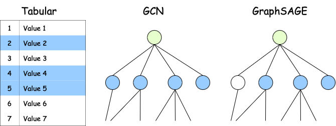
With tabular data, sampling is easy. It is something you do in all common automatic learning projects by creating trains, testing and validation sets. With graphics, you cannot select random nodes. This can lead to disconnected graphics, nodes without neighbors, etc.:

That you can Making graphics is to select a subset of random fixed fixed neighbors. For example, in a social network, you can try 3 friends for each user (instead of all friends):

2. Added information

After the neighbor's selection of the previous part, Graphsage combines its characteristics in a single representation. There are multiple ways to do this (multiple aggregation functions). The most common types and those explained on paper are Medium aggregation, LSTMand group.

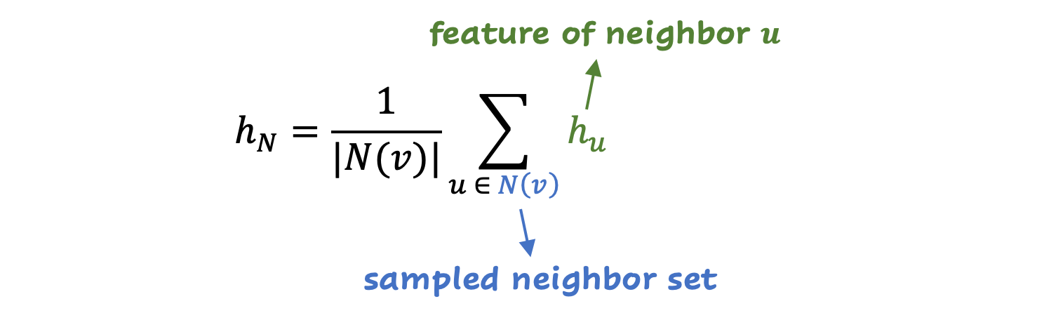
With the average aggregation, the average is calculated in all the characteristics of the sampled neighbors (very simple already effective). In a formula:

LSTM aggregation uses a LSTM (neuronal network type) to process the characteristics of neighbors sequentially. It can capture more complex relationships, and is more powerful than average aggregation.

The third type, group aggregation, applies a non -linear function to extract key characteristics (think of Polvocanado in a neuronal network, where it also takes the maximum value of some values).

3. Update the node representation

After sampling and aggregation, the node . The nodes will learn from their neighbors, but they will also maintain their own identity, as we saw before with GCNS and GATS. Information can flow through the graph effectively.

This is the formula for this step:

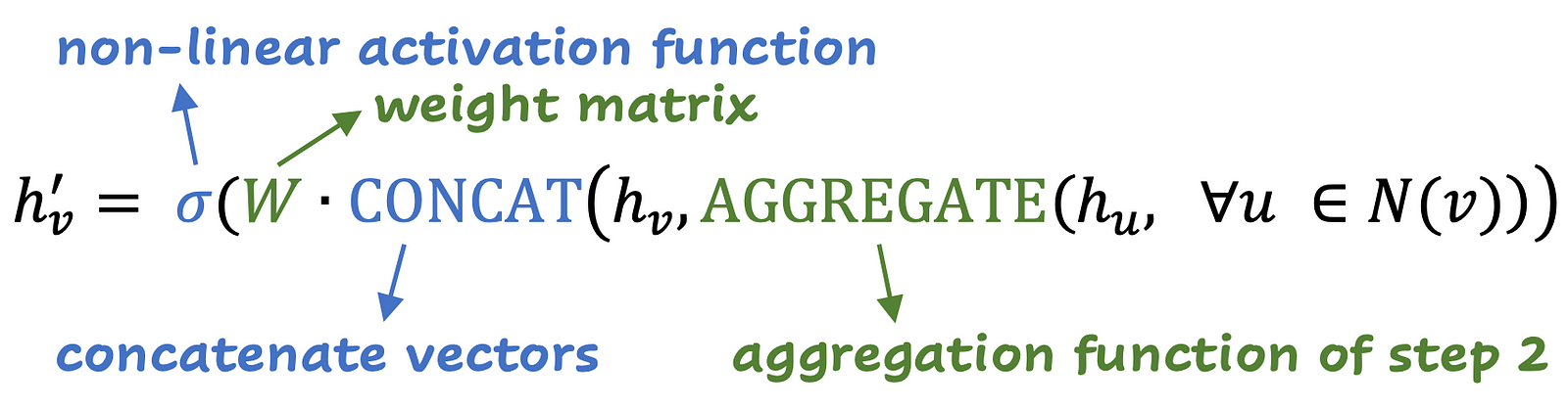
The aggregation of step 2 is done on all neighbors, and then the representation of node characteristics is concatenated. This vector is multiplied by the weight matrix and passes through the non -linearity (for example, reluct). As a final step, normalization can be applied.

4. Repeat for multiple layers

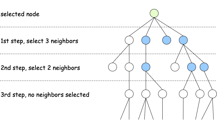
The first three steps can be repeated several times, when this happens, the information can flow from distant neighbors. In the image below, see a node with three neighbors selected in the first layer (direct neighbors) and two neighbors selected in the second layer (neighbors of neighbors).

To summarize, Graphsage's key forces are scalability (sampling makes it efficient for mass graphics); flexibility, you can use it for inductive learning (it works well when used to predict in invisible nodes and graphics); The aggregation helps with generalization because it softens noisy characteristics; and the multiple layers allow the model to learn from distant nodes.

Cool! And the best, Graphsage is implemented in PygSo we can easily use it in Pytorch.

Predict with Graphsage

In the previous publications, we implement a MLP, GCN and GAT in the CORA Dataset (CC by-sa). To refresh your mind, CORA is a set of data with scientific publications in which the subject of each article must predict, with seven classes in total. This data set is relatively small, so it might not be the best set to try Graphsage. We will do this anyway, just to be able to compare. Let's see how well Graphsage works.

Interesting parties of the code that I like to highlight Graphsage:

• He NeighborLoader that performs the selection of the neighbors for each layer:

from torch_geometric.loader import NeighborLoader

# 10 neighbors sampled in the first layer, 10 in the second layer
num_neighbors = (10, 10)

# sample data from the train set
train_loader = NeighborLoader(
    data,
    num_neighbors=num_neighbors,
    batch_size=batch_size,
    input_nodes=data.train_mask,
)

• The type of aggregation is implemented in the SAGEConv layer. The default value is meanYou can change this to max either lstm:

from torch_geometric.nn import SAGEConv

SAGEConv(in_c, out_c, aggr='mean')

• Another important difference is that Graphsage is trained in mini lots, and GCN and GAT in the complete data set. This touches the essence of Graphsage, because Graphsage's neighboring sampling makes it possible to train in mini lots, we no longer need the complete graph. The GCN and the GAT need the complete graph for the spread of correct characteristics and the calculation of the care scores, so we train GCN and GATS in the complete chart.
• The rest of the code is similar to the before, except that we have a class where all different models are instant in a function of model_type (GCN, GAT or SAGE). This makes it easy to compare or make small changes.

This is the complete script, we train 100 times and repeat the experiment 10 times to calculate the average precision and the standard deviation for each model:

import torch
import torch.nn.functional as F
from torch_geometric.nn import SAGEConv, GCNConv, GATConv
from torch_geometric.datasets import Planetoid
from torch_geometric.loader import NeighborLoader

# dataset_name can be 'Cora', 'CiteSeer', 'PubMed'
dataset_name = 'Cora'
hidden_dim = 64
num_layers = 2
num_neighbors = (10, 10)
batch_size = 128
num_epochs = 100
model_types = ('GCN', 'GAT', 'SAGE')

dataset = Planetoid(root='data', name=dataset_name)
data = dataset(0)
device = torch.device('cuda' if torch.cuda.is_available() else 'cpu')
data = data.to(device)

class GNN(torch.nn.Module):
    def __init__(self, in_channels, hidden_channels, out_channels, num_layers, model_type='SAGE', gat_heads=8):
        super().__init__()
        self.convs = torch.nn.ModuleList()
        self.model_type = model_type
        self.gat_heads = gat_heads

        def get_conv(in_c, out_c, is_final=False):
            if model_type == 'GCN':
                return GCNConv(in_c, out_c)
            elif model_type == 'GAT':
                heads = 1 if is_final else gat_heads
                concat = False if is_final else True
                return GATConv(in_c, out_c, heads=heads, concat=concat)
            else:
                return SAGEConv(in_c, out_c, aggr='mean')

        if model_type == 'GAT':
            self.convs.append(get_conv(in_channels, hidden_channels))
            in_dim = hidden_channels * gat_heads
            for _ in range(num_layers - 2):
                self.convs.append(get_conv(in_dim, hidden_channels))
                in_dim = hidden_channels * gat_heads
            self.convs.append(get_conv(in_dim, out_channels, is_final=True))
        else:
            self.convs.append(get_conv(in_channels, hidden_channels))
            for _ in range(num_layers - 2):
                self.convs.append(get_conv(hidden_channels, hidden_channels))
            self.convs.append(get_conv(hidden_channels, out_channels))

    def forward(self, x, edge_index):
        for conv in self.convs(:-1):
            x = F.relu(conv(x, edge_index))
        x = self.convs(-1)(x, edge_index)
        return x

@torch.no_grad()
def test(model):
    model.eval()
    out = model(data.x, data.edge_index)
    pred = out.argmax(dim=1)
    accs = ()
    for mask in (data.train_mask, data.val_mask, data.test_mask):
        accs.append(int((pred(mask) == data.y(mask)).sum()) / int(mask.sum()))
    return accs

results = {}

for model_type in model_types:
    print(f'Training {model_type}')
    results(model_type) = ()

    for i in range(10):
        model = GNN(dataset.num_features, hidden_dim, dataset.num_classes, num_layers, model_type, gat_heads=8).to(device)
        optimizer = torch.optim.Adam(model.parameters(), lr=0.01, weight_decay=5e-4)

        if model_type == 'SAGE':
            train_loader = NeighborLoader(
                data,
                num_neighbors=num_neighbors,
                batch_size=batch_size,
                input_nodes=data.train_mask,
            )

            def train():
                model.train()
                total_loss = 0
                for batch in train_loader:
                    batch = batch.to(device)
                    optimizer.zero_grad()
                    out = model(batch.x, batch.edge_index)
                    loss = F.cross_entropy(out, batch.y(:out.size(0)))
                    loss.backward()
                    optimizer.step()
                    total_loss += loss.item()
                return total_loss / len(train_loader)

        else:
            def train():
                model.train()
                optimizer.zero_grad()
                out = model(data.x, data.edge_index)
                loss = F.cross_entropy(out(data.train_mask), data.y(data.train_mask))
                loss.backward()
                optimizer.step()
                return loss.item()

        best_val_acc = 0
        best_test_acc = 0
        for epoch in range(1, num_epochs + 1):
            loss = train()
            train_acc, val_acc, test_acc = test(model)
            if val_acc > best_val_acc:
                best_val_acc = val_acc
                best_test_acc = test_acc
            if epoch % 10 == 0:
                print(f'Epoch {epoch:02d} | Loss: {loss:.4f} | Train: {train_acc:.4f} | Val: {val_acc:.4f} | Test: {test_acc:.4f}')

        results(model_type).append((best_val_acc, best_test_acc))

for model_name, model_results in results.items():
    model_results = torch.tensor(model_results)
    print(f'{model_name} Val Accuracy: {model_results(:, 0).mean():.3f} ± {model_results(:, 0).std():.3f}')
    print(f'{model_name} Test Accuracy: {model_results(:, 1).mean():.3f} ± {model_results(:, 1).std():.3f}')

And here are the results:

GCN Val Accuracy: 0.791 ± 0.007
GCN Test Accuracy: 0.806 ± 0.006
GAT Val Accuracy: 0.790 ± 0.007
GAT Test Accuracy: 0.800 ± 0.004
SAGE Val Accuracy: 0.899 ± 0.005
SAGE Test Accuracy: 0.907 ± 0.004

Awesome improvement! ¡Incluso en este pequeño conjunto de datos, Graphsage supera a GAT y GCN fácilmente! I repeated this test for data sets from Citaseer and Pubmed, and always Graphsage came better.

What I like to point out here is that GCN is still very useful, it is one of the most effective baselines (if the structure of the graph allows). In addition, I did not do much tuning of hyperparameter, but I only went with some standard values ​​(such as 8 heads for multi-coat gat attention). In larger, more complex and noisy graphics, Graphsage's advantages become clearer than in this example. We did not do any performance test, because for these graphsage small graphics it is not faster than GCN.

Conclusion

Graphsage brings us very pleasant improvements and benefits compared to Gats and GCNS. Inductive learning is possible, Graphsage can handle changing graphic structures quite well. And we do not try it in this publication, but the sampling of neighbors makes it possible to create representations of characteristics for larger graphics with good performance.

Related

Connection optimization: mathematical optimization within the graphics

Graphic Neural Networks Part 1. Graphic Convolucional Networks explained

Graphic Neural Networks Part 2. Graphics Care Networks vs. GCNS