In early 2024, Brazil experienced heavy rainfall, particularly in the south and northeast regions, leading to floods that damaged cities, destroyed crops, and caused fatalities. As climate change increases the frequency of extreme weather conditions, such as droughts and floods, contingency planning and risk assessment are becoming increasingly crucial for managing such events.
This article presents a Python and Jupyter Notebook workflow for Flood Risk assessment in rural and small-city areas of a northeastern Brazilian state. The process begins with a digital elevation model (DEM) and ends with a visualization of the likelihood of inundation of different areas using the Height Above Nearest Drainage (HAND) model. The method aims to assess flood risk in inner-city areas in real time and with little data and computational resources.
Overview
- How do you find and download DEM data for flood inundation risk analysis?
- How do you set the programming environment with the necessary packages for the analysis?
- How do data preparation and pre-processing steps for DEM files for drainage extraction be performed?
- How to use the HAND model to identify the risk of inundation of different areas and label them as “very high risk”, “high risk”, “moderate risk”, “low risk”, and “very low risk”.
Setting the Environment
The workflow used for the analysis presented in this study is available here. The workflow is a Jupyter Notebook that runs on Python 3.12 and uses the following packages:
- Numpy – array manipulation.
- Whiteboxtools – Geospatial analysis and manipulation.
- GDAL – Geospatial data manipulation.
- RichDEM – DEM and hydrological analysis tools.
- Matplotlib – Data Visualization.
Data Preparation and Acquisition
For Flood Risk assessment, here are the data preparations and acquisition steps:
Step 1: Data Acquisition
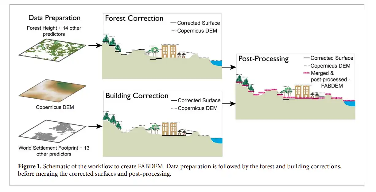
The first step is acquiring elevation data for the area of interest. This study uses DEM files from FABDEM (Forest and Buildings Removed Copernicus DEM), which are publicly available on the University of Bristol’s website (1). FABDEM is a global elevation map that removes building and tree height biases from the Copernicus GLO-30 Digital Elevation Model (DEM). The data is provided at a resolution of 1 arc second (approximately 30 meters at the equator) for the entire globe.
As previously mentioned, this study’s area of interest is Brazil’s northeast region. The DEM file covers a 1º-by-1º area, ranging from 6ºS 39ºW to 5ºS 38ºW, using the WGS84 coordinate system (EPSG: 4326). This region is illustrated in Figure 1 below.
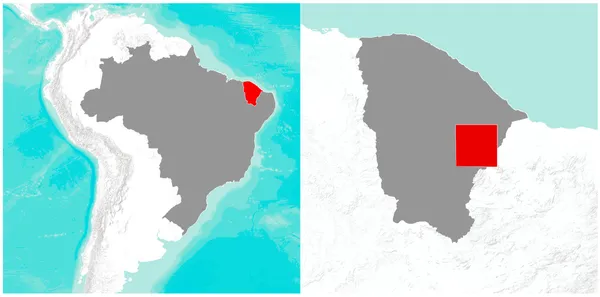
The highlighted area lies within one of Brazil’s most arid biomes. It is characterized by an irregular and sparse rainfall pattern, with rain typically falling only a few months per year. However, in 2024, this region suffered from an unusually high volume of rainfall concentrated over a short period, significantly impacting the area.
Step 2: Data Preparation
The data preparation consists of filling the DEM file’s sinks. Sinks are areas where elevation data forms a depression; in other words, they are pixels or sets of pixels that have neighbouring pixels with higher elevation. In hydrology analysis, water is collected in sinks instead of flowing.
While sinks are natural features, like lakes and basins, they can be created by DEM errors, such as low resolution or data collection. Therefore, these depressions or sinks are “filled” during preprocessing to ensure smooth water flow by either removing them or raising their elevation so that the hydrological modelling remains unaffected. This is an important step in performing Flood Risk Assessment, among other hydrological studies.
This step will use Python libraries such as WhiteboxTools and RichDEM to ensure the DEM is processed to represent a smooth surface suitable for accurately calculating flow direction and flow accumulation.
Also read: Geospatial Analysis for Flood Resilience
Flow Direction and Flow Accumulation
Calculating Flow Directions
The next step involves determining the flow direction for each pixel in the DEM. This creates a new raster where each pixel’s value represents the flow direction. There are three methods: D8, Multiple Flow Direction (MFD), and D-Infinity (DINF).
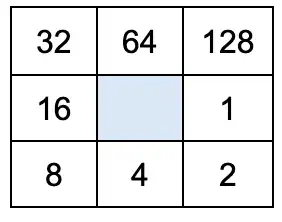
This study uses the D8 method, which models flow direction by finding the steepest downslope neighbour for each pixel. The resulting raster contains values between 1 and 128, indicating flow direction based on the steepest descent. For example, if the steepest slope is to the right, the pixel’s value will be 1, and if it’s toward the upper-right corner, the value will be 128, as shown in the diagram below.
Calculating Flow Accumulation
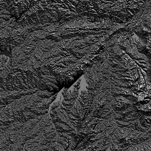
Once the flow direction has been calculated, the next step is to compute the flow accumulation. Flow accumulation identifies the areas where water is likely to collect based on the flow direction. This is achieved by determining the number of upstream pixels contributing to each pixel’s flow.
The output is a new raster where the value of each pixel represents the total accumulated flow at that location. Pixels with high accumulation values typically correspond to streams, rivers, or drainage networks as they gather flow from multiple upstream areas. Conversely, pixels with low accumulation values indicate areas such as ridges or elevated terrain with minimal water accumulation, as illustrated in Figure 3.
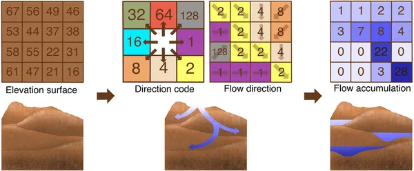
With Python, flow accumulation can be calculated with the WhiteboxTools using the d8_flow_accumulation method.
Using the flow accumulation raster, it is possible to identify areas representing watercourses, such as rivers, streams, and drainage networks. This is achieved by applying a threshold to the accumulation values, where any pixel with a value above the threshold is considered part of the stream network.
The choice of the threshold value depends on several factors, such as the hydrological conditions of the study area and the resolution of the DEM. In this case, the region is predominantly semi-arid, and the DEM has a spatial resolution of 30 meters. After some trial and error, a threshold value of 15 was considered most suitable for capturing broader drainage networks.
HAND Model Analysis
HAND (Height Above Nearest Drainage) analysis, first introduced by NOBRE et al. (2011), is a method used to assess an area’s susceptibility to flood inundation. This is done by utilizing a DEM (Digital Elevation Model) and a stream network raster to determine how high each DEM pixel is above the stream network’s nearest pixel. The result is a new raster where each pixel value represents the vertical distance between the pixel’s elevation and the elevation of the closest drainage point, as illustrated in Figure 4.

The pixel values in the resulting HAND raster represent the relative height above the nearest drainage point. Higher values indicate areas farther from the drainage, which are less likely to flood, while lower values represent areas closer to the drainage, making them more susceptible to flooding.
This analysis generated the HAND raster using the WhiteboxTools Python library and the elevation_above_stream method. The resulting raster contains pixel values ranging from 0 to 330 meters, representing the height of each DEM pixel above the nearest drainage point in the study area.
Classifying Flood Risk With HAND Model
Based on the pixel values from the HAND raster, risk classes can be defined, with lower values indicating a higher risk of inundation compared to areas with greater elevation. Table 1 below presents the thresholds (in meters) used to classify regions into different risk levels.
Table 1: Intervals used to classify risk levels.
| Risk Level | Threshold (m) | Class Value |
|---|---|---|
| Very High | 0 – 1 | 5 |
| High | 1 – 2 | 4 |
| Medium | 2 – 6 | 3 |
| Low | 6 – 10 | 2 |
| Very Low | 10 | 1 |
The thresholds presented in Table 1 were determined through empirical testing. Using the NumPy package, class values can be assigned to different regions of the original DEM, and a new raster file can be generated with the classification results.
The thresholds presented in Table 1 were determined through empirical testing. Using the NumPy package, class values can be assigned to different regions of the original DEM, and a new raster file can be generated with the classification results.
Results and Discussions
With all the processing steps completed, it’s time to visualize the results and reach some conclusions. The Matplotlib Python package allows you to visualize the results of the risk classification of the HAND raster file, as presented in Figure 5.
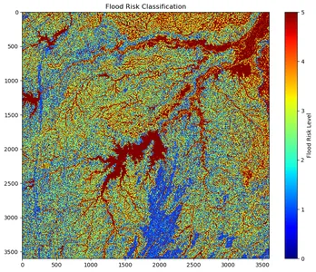
To better understand which regions are more prone to flooding, the GDAL Python library can be used to export the classified array as a GeoTIFF file. This file can then be loaded into GIS software, such as QGIS, to visualize the higher-risk areas, as illustrated in Figure 6 below.
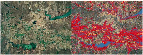
In Figure 6, a rural area is shown with a small city located in the centre. On the right side of the figure, high-risk regions (highlighted in yellow) and very high-risk areas (highlighted in red) are indicated. The stream network, represented in blue, shows the extent of areas near the streams at risk of inundation.
Conclusion
The HAND model is very useful for assessing the risk of inundation of areas quickly and computationally efficiently. Using only a DEM file from an area of interest, it is possible to map (Flood Risk assessment) areas prone to inundation and facilitate the development of contingency plans to mitigate the impacts. The workflow proposed in the present study can be used for different areas and situations, and it is advantageous for civil security agencies.
The Jupyter Notebook with all the steps, detailed explanations, and requirements is available here.
References
- Nathan, Smiti & Harrower, Michael. (2023). Mapping spatial patterning of Bronze Age towers in Oman according to water flow accumulation. Arabian Archaeology and Epigraphy. 34. n/a-n/a. 10.1111/aae.12237.
- Hu, Anson & Demir, Ibrahim. (2021). Real-Time Flood Mapping on Client-Side Web Systems Using HAND Model. Hydrology. 8. 65. 10.3390/hydrology8020065.
- Nobre, A.D., Cuartas, L.A., Hodnett, M., Rennó, C.D., Rodrigues, G., Silveira, A., Waterloo, M., Saleska, S., Height above the Nearest Drainage, a hydrologically relevant new terrain model, Journal of Hydrology (2011), doi: 10.1016/j.jhydrol.2011.03.05.1
- Lindsay, J.B. (2023). Introduction to WhiteboxTools: A User Guide for the WhiteboxTools Command-Line Interface and Python API. Whitebox Geospatial Inc. Retrieved from Whiteboxgeo.
- Barnes, R. (2023). RichDEM: High-performance Terrain Analysis Library for Digital Elevation Models. Retrieved from RichDEM — High-Performance Terrain Analysis.
- Esri. (2024). Understanding Drainage Systems. ArcGIS Pro. Retrieved from Understanding drainage systems—ArcGIS Pro.
Frequently Asked Questions
Ans. The present study used FABDEM with a resolution of 30 meters. While it is useful for larger areas, lower-resolution DEMs tend to generalize terrain features, leading to inaccuracies in the stream extraction step and, consequently, misclassification of areas concerning flood risk.
Ans. In this study, we tested various options to choose the threshold value for stream network extraction. Higher threshold values create smaller drainage areas, making the extracted stream network look different from satellite imagery. Therefore, it’s important to select a threshold that produces a drainage network closely matching the water features visible in the imagery of the area of interest.
Ans. The HAND model indicates that high-risk (yellow) and very high-risk (red) areas are more flood-prone due to their proximity to the drainage network. However, classifying an area as flooded also requires considering factors like land use, precipitation patterns, and historical flood data.
Ans. The proposed workflow enables real-time mapping of flood-prone areas, enhancing situational awareness, mitigation, and emergency response. The HAND model offers a practical, scalable solution using only DEM data and open-source Python libraries, making it ideal for regions with limited technological resources to assess flood risks reliably.
 NEWSLETTER


