Introduction
Vector databases have been the fastest-growing database category for a few years, with their relevance growing more in the era of Generative ai. What differentiates them from relational databases is the implementation of ANN algorithms. What are they, you ask? Well, this article will explain what ANN algorithms in vector databases are and how they work. Moreover, it will discuss their unique methods for efficient data searching and practical applications across various industries. So, let’s begin.
Learn More: Vector Databases in Generative ai Solutions
Learning Objectives
- Learn how data representation and search methods differ between relational and vector databases, highlighting the limitations of binary search in multi-dimensional spaces.
- Gain insights into tree-based ANN algorithms such as KD-trees and the Annoy library’s method of dividing data points using random hyperplanes.
- Understand graph-based ANN algorithms, especially the HNSW algorithm, and how they efficiently construct and navigate graphs to find nearest neighbors.
- Explore hybrid algorithms like NGT, which enhance search speed and accuracy by integrating tree and graph structures.
- Discover the practical applications of vector databases in music recommendations, product recommendations, personalized advertising, and more.
What are ANN Algorithms?
In relational databases, each record is represented in a row and its attributes are represented in columns. For instance, consider a table with N author names and their respective research paper data. A naive approach would compare the query author’s name to all N values in the Author column to find the books written by a particular author. This method requires N comparisons.
A more efficient method is sorting the Author column alphabetically. Then by using binary search, we can find using only log(N) comparisons. However, the scenario changes when it comes to finding relevant research papers based on a given query. The naive approach is to find the similarity between the query embedding vector and all the document embedding vectors, requiring N comparisons.
Sorting the research paper text or embeddings and using binary search doesn’t work because we are not looking for the exact match to the query embedding. We only want to find the most similar embeddings. Moreover, embeddings represent the data in multi-dimensional space. Sorting by any single dimension doesn’t make sense.
So, we need different algorithms that can search for vectors more efficiently. These algorithms are called Approximate Nearest neighbor (ANN) algorithms. While these algorithms may not always find the most precise nearest neighbors compared to the naive approach, they significantly improve search speed and efficiency in large, multi-dimensional datasets. The implementation of ANN algorithms is what differentiates vector databases from traditional relational databases.
Learn More: Top 15 Vector Databases in 2024
How ANN Algorithms Work
Now that you understand what ANN algorithms are, let’s find out how different ANN algorithms work.
Tree-based Algorithms
Tree-based algorithms organize data points where points that are closer in space are also closer in the tree. A few examples of such trees are the K-dimensional tree (KD-tree), Vantage Point tree (VP-tree), Ball tree, and Rectangular tree (R-tree).
One popular library that implements a tree-based algorithm is Annoy (Approximate Nearest Neighbors Oh Yeah). It was developed by Erik Bernhardsson while working at Spotify. Annoy builds the tree by dividing data points using random hyperplanes.
Let’s look into the details of how this works.

How Annoy Works
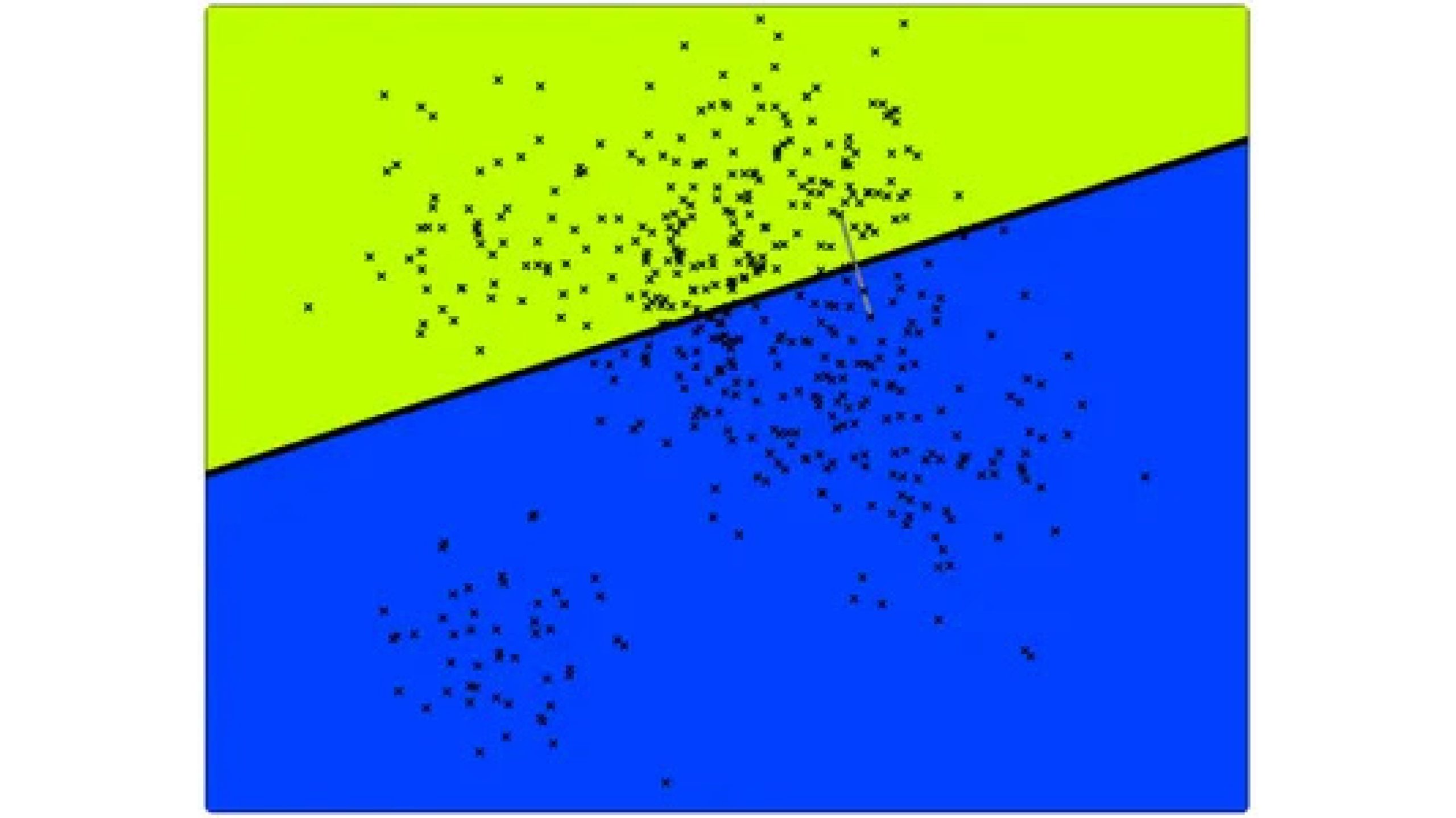
- Consider all the points located in the space as shown in the image.
- Randomly choose two points from the dataset.
- Calculate a hyperplane that is perpendicular to the line segment connecting the two points and passes through the midpoint of the line segment. We can use this hyperplane to divide all the points to the left or right side of the tree node.
- Take the normal vector of the hyperplane and calculate the dot product with each data point. If the dot product is positive, the point is in the same direction as the normal vector. If the dot product is negative, the point is in the opposite direction as the normal vector. Based on the dot product, split the points into left or right child nodes.
- Recursively split nodes by hyperplanes until only a few points remain in the leaf nodes. This divides the total space into grids, where leaf nodes store the points and all other nodes store the hyperplanes used for division.
- To find the nearest neighbors for a query point, calculate its dot product with the normal vector of the root node hyperplane. Based on the result, traverse either to the left or right of the node. Continue traversing until reaching the leaf node. Then, calculate the similarity between the query and the points in the leaf node.
- As the tree is a binary tree, finding nearest neighbors requires approximately log(N) comparisons.
- If the query point is near the edge of any grid, considering only one leaf node may miss similar points in adjacent leaf nodes. To address this, we can build multiple trees, each with different random starting points, thus different hyperplanes. Traverse each tree with the query and calculate similarity with points in the leaf nodes of all trees, ensuring not to miss any nearest neighbor.
- We can also store the nodes with calculated similarities in a priority queue to return the top-k nearest neighbors.
This detailed description explains how tree-based ANN algorithms work, particularly in dividing data points and finding nearest neighbors efficiently. By considering edge cases and utilizing multiple trees, the algorithm can improve accuracy and performance in finding the nearest neighbors.
Graph-based Algorithms
In these algorithms, data points are represented as vertices of the graph, and edges are used to traverse the graph to find nearest neighbors. Let’s understand it in detail using the most popular algorithm currently, Hierarchical Navigable Small World (HNSW).

How HNSW Works
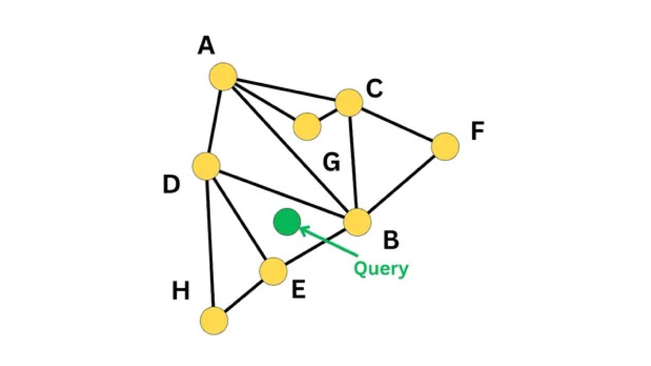
- As shown in the above image, each vertex in the graph represents a data point.
- Connect each vertex with a configurable number of nearest vertices in a greedy manner.
- To find the nearest neighbors for a query, start from any random vertex, say A.
- Find the vertices connected to A, which might be C, G, and D.
- Calculate the distance between the query and each of these vertices (A, C, G, D).
- Compare the distances and move to the vertex closest to the query, which is D in this case.
- Repeat this process with vertex D and its connected vertices, moving next to E.
- When we repeat this process by starting at E, we find that E is the closest vertex to the Query again. So, we found the nearest neighbor to our query.
If you are wondering how we have built the graph in the first place, just like we have found the nearest neighbors for a query, we can find the nearest neighbors for a new vertex as we are inserting it. Then we can connect the new vertex to pre-defined nearest vertices through edges.
In the graph, each vertex connects to only a few nearby vertices, thereby creating a small-world network. As we navigate it, this is called a navigable small world.
When dealing with millions of data points, traversing the graph to find the nearest neighbor starting from a random point can be time-consuming, as each vertex is connected to only a few vertices. Increasing the number of edges for each vertex also takes a lot of time as more distances need to be calculated.
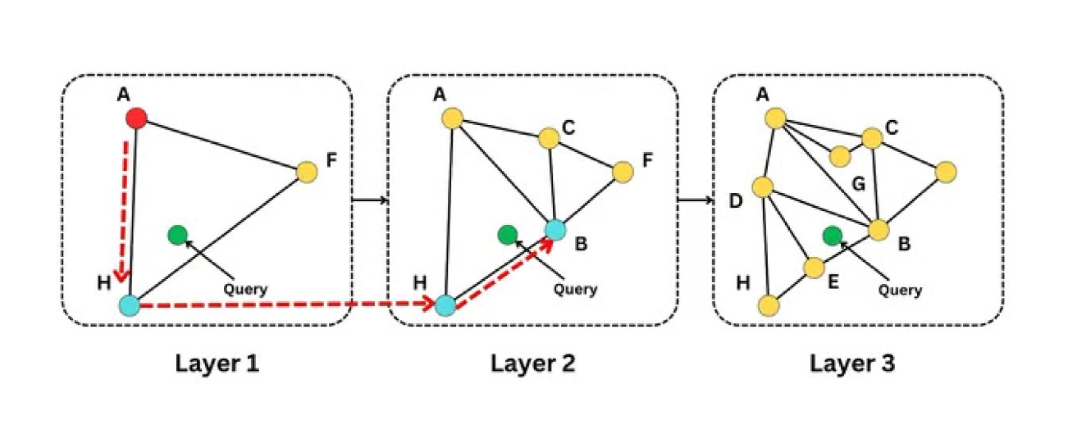
To overcome this problem, multiple graphs with different numbers of vertices are built. Each graph can be considered a layer.

How This Works
- In the first layer, use a fraction of the data points to build the graph, for example, N/4.
- In the next layer, use N/2 data points to build the graph.
- In the last layer, use all the data points.
- To find the nearest neighbors to the query, start from layer 1.
- Since the number of vertices is fewer, the edges are longer, allowing quick traversal to a nearer vertex in that layer (for example, H).
- Start from vertex H in the next layer and traverse the graph until the nearest neighbor in that layer is found (vertex B).
- Continue this process until the nearest neighbor is found in the last layer.
Thus, the number of traversals and distance calculations are fewer as compared to the NSW algorithm.
HNSW Formula and Implementation
How do we decide the number of layers and how many data points should be in each? The HNSW paper provides the following formula for allocating data points to different layers.
floor(-ln(unif(0,1))*mL)
Here,
- unif(0,1) represents a random number drawn from a uniform distribution between 0 and 1.
- −ln(unif(0,1)) natural logarithm of a uniform random number is used to transform the uniform distribution into an exponential distribution. This transformation along with -ve sign makes it the right-skewed distribution.
- mL is a multiplier that scales the logarithmic value. It is usually set to 1/ln(M), where M is the maximum number of neighbors each node can have.
- The floor function rounds down the resulting value to the nearest integer. This determines the discrete level at which the node will be placed.
HNSW is the default algorithm for most of the vector databases. Spotify also released a new library Voyager based on HNSW.
Now, let’s try the HNSW algorithm
import numpy as np
import faiss

# We can choose some random numbers for the database and queries.
d = 256                           # dimension
nb = 100000                      # database size
nq = 10000                       # number of queries
np.random.seed(1234)             # make reproducible
xb = np.random.random((nb, d)).astype('float32')
xb(:, 0) += np.arange(nb) / 1000.
xq = np.random.random((nq, d)).astype('float32')
xq(:, 0) += np.arange(nq) / 1000.
First, let’s try the naive approach by building the FlatIndex.
flat_index = faiss.IndexFlatL2(d)   # build the index
print(flat_index.is_trained)
>>> True

flat_index.add(xb)                  # add vectors to the index
print(flat_index.ntotal)
>>> 100000
Now, we can search
%%time            # this command will give time taken to run in jupyter notebook
k = 5                             # we can get 5 nearest neighbors
D, I = flat_index.search(xq, k)     # actual search
print(I(:5))                   # neighbors of the 5 first queries
print(D(:5))                   # distances of the 5 first queries

>>>((  69  525  628  595 1413)
 ( 603   25   14 1616  698)
 ( 732  744  739  589 1185)
 ( 447  841  347  373  631)
 (1053  924  163  101  302))
((33.871002 33.979095 34.67044  34.738922 35.204865)
 (34.497314 34.682297 35.488464 35.671005 35.864685)
 (32.993195 34.401352 34.411896 34.514572 34.659515)
 (33.948517 34.039062 34.364456 34.466248 35.244644)
 (33.487595 34.77111  34.81253  34.893692 35.152557))
Lt’s try the HNSW algorithm now
M = 32              # each vertex will be connected to M other nearest vertices
hnsw_index = faiss.IndexHNSWFlat(d, M)   # build the index
print(hnsw_index.is_trained)

>>> True
We can add the data to the index.
# To connect to M other vertices, it will greedily search upto 'efConstruction' vertices.
# the default value is 40, we can change it before adding dataset
hnsw_index.hnsw.efConstruction = 48

hnsw_index.add(xb)

# after adding our data we will find that the level has been set automatically
hnsw_index.hnsw.max_level
>>> 3

# and levels (or layers) are now populated
levels = faiss.vector_to_array(hnsw_index.hnsw.levels)
np.bincount(levels)
>>> array((    0, 96812,  3093,    92,     3))
We can search now
# how many entry points will be explored between layers during the search.
# for example, we can select 30 nearest vertices in one layer,
# then start traversing the graph from those vertices in the next layer
hnsw_index.hnsw.efSearch = 30

%%time
hnsw_index.search(xq(:5), k=4)

>>> (array(((33.870995, 33.979073, 34.67042 , 34.738907),
        (34.497334, 34.682304, 35.488453, 35.67101 ),
        (32.993187, 34.401337, 34.411903, 34.514584),
        (33.948494, 34.039097, 34.36444 , 34.46623 ),
        (33.487595, 34.771133, 34.81257 , 34.893723)), dtype=float32),
 array(((  69,  525,  628,  595),
        ( 603,   25,   14, 1616),
        ( 732,  744,  739,  589),
        ( 447,  841,  347,  373),
        (1053,  924,  163,  101))))
Hybrid Algorithms
In these algorithms, we use both trees and graphs to find the nearest neighbors. An example is Neighborhood Graph and Tree (NGT) which is the best-performing ANN algorithm currently. NGT uses a dynamic vantage point tree and a graph. Let’s see how it works.

How NGT Works
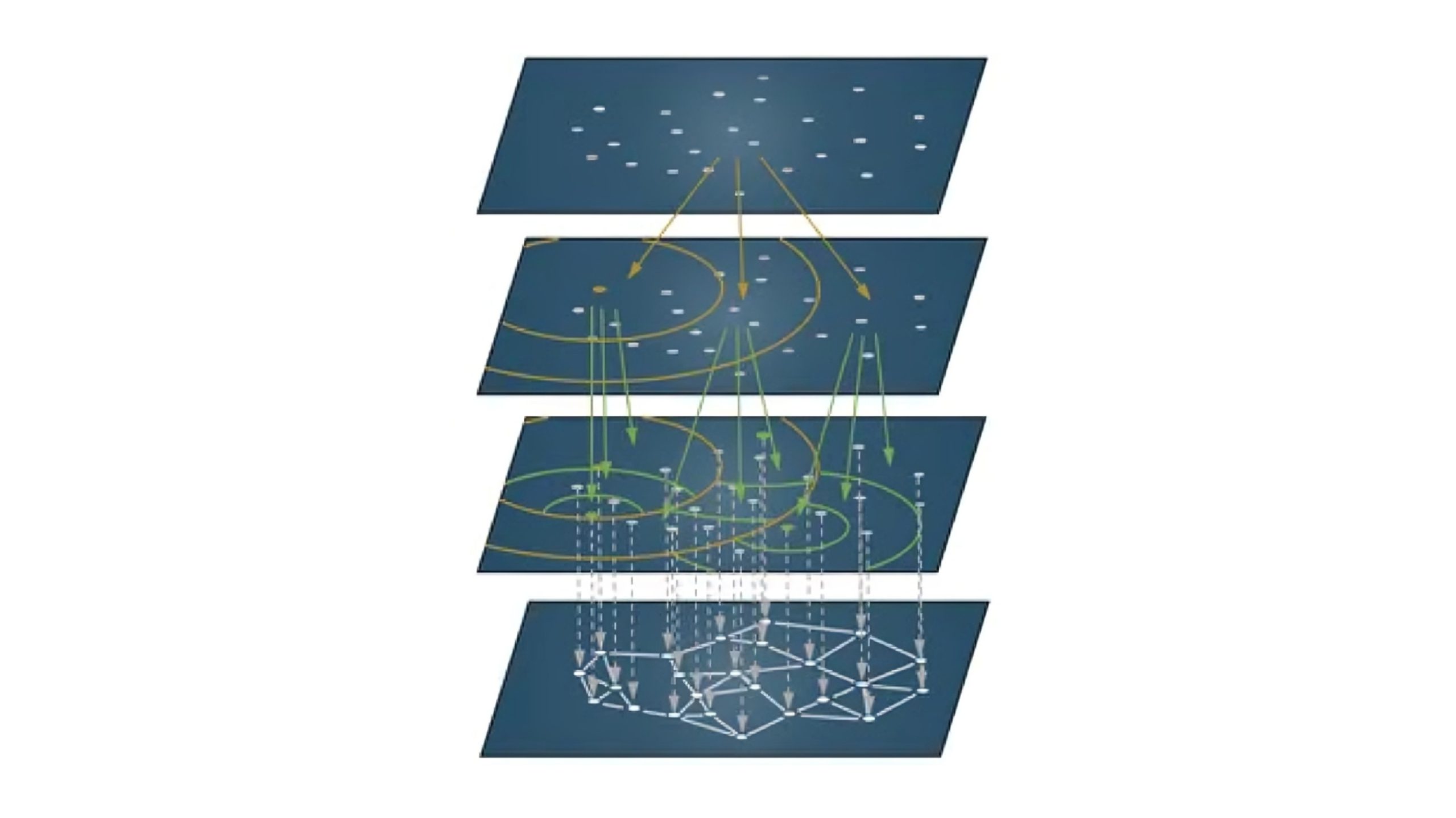
- The dvp-tree begins with a single leaf node representing the entire data space as shown in the above image.
- As we add new points, the tree traverses to find the appropriate leaf node for insertion.
- When the number of points in a leaf node exceeds a predefined maximum, the leaf node is split into smaller subspaces. This splitting is similar to the vantage point tree (vp-tree) method, where a vantage point is chosen, and the space is divided using hyperspheres centered at this vantage point.
- For each point in the node, we calculate the distance to the vantage point.
- Choose a radius ‘r’ such that it balances the points between inside and outside the hypersphere.
- Points with a distance d≤r from the vantage point are inside the hypersphere, and points with d>r are outside. The circles and arcs in the above image represent these hyperspheres.
- This division process is repeated recursively, creating a hierarchical structure of nodes and subnodes.
- The dvp-tree supports dynamic updates, meaning we can incrementally add points without reconstructing the entire tree.
- The process continues until each leaf node contains a manageable number of points.
- Then, we can traverse only the leaf nodes in a graph using the NSW algorithm as explained above.
So, rather than traversing all the nodes using a graph using HNSW, we are localizing the search space using a dynamic vantage point tree in this algorithm. This combination of using both tree and graph makes it one of the fastest and most accurate algorithms. As of June 2024, Vald vector database supports this algorithm.
Applications of ANN Algorithms in Vector Databases
Let’s now explore some of the most common applications of ANN algorithms.
1. Similarity-Based Recommendations
These applications focus on finding approximate matches to user preferences or content features.
- Music Recommendations: Platforms like Spotify use vector databases to recommend music based on user listening habits and song features. That’s why Spotify developed those ANN libraries.
- Product Recommendations: E-commerce sites use vector databases to suggest products similar to those a user has viewed or purchased.
- Personalized Advertising: Vector databases match ads to users based on their behavior and preferences, improving engagement and conversion rates. It is Yahoo Japan which developed the NGT algorithm.
2. Embedding-Based Search
These applications utilize embeddings to search for similar items across various media types, enhancing search accuracy and relevance.
- Text Search: In natural language processing, vector databases store text embeddings for semantic search, document retrieval, and question-answering systems
- Image and Video Search: Allow for the retrieval of visually similar images, used in reverse image search, content-based image or video retrieval, and digital asset management.
- Molecule Search: In bioinformatics and drug discovery, molecule embeddings help find structurally similar molecules, supporting the identification of potential drug candidates.
3. Miscellaneous
- Other applications include anomaly detection, geospatial analysis, etc.
Learn More: 10+ Vector Database Applications in the Real World
Conclusion
Vector databases, through efficient ANN algorithms like tree-based, graph-based, and hybrid methods, significantly enhance search capabilities in multi-dimensional spaces. Their practical applications span various industries, offering powerful solutions for similarity-based recommendations, embedding-based search, and personalized advertising.
Hope this article has given you a detailed idea of ANN algorithms in vector databases. Do check out our other articles on vector databases to learn more. Happy learning!
Key Takeaways
- Vector databases excel in handling multi-dimensional data searches, surpassing traditional relational databases in efficiency and speed.
- Tree-based ANN algorithms like KD-trees and Annoy improve search performance by organizing data points using random hyperplanes.
- Graph-based algorithms, such as HNSW, effectively navigate complex data spaces by connecting data points through vertices and edges
- Hybrid algorithms like NGT combine the strengths of trees and graphs to achieve faster and more accurate nearest neighbor searches.
- Vector databases are crucial in applications like recommendations, personalized advertising, and embedding-based search across various media types.
Frequently Asked Questions
A. A vector database is a specialized type of database that handles multi-dimensional data, enabling efficient similarity searches using vector embeddings rather than traditional row-column structures.
A. Vector databases utilize various Approximate Nearest Neighbor (ANN) algorithms, including tree-based methods like KD-trees and Annoy, graph-based methods like HNSW, and hybrid methods like NGT.
A. Tree-based ANN algorithms organize data points using structures like KD-trees and Annoy, which divide the data space with hyperplanes, allowing efficient nearest neighbor searches by traversing the tree.
A. Graph-based algorithms, such as HNSW, represent data points as vertices in a graph, using edges to connect nearest neighbors and navigate the graph efficiently to find similar data points.
A. Practical applications of vector databases include similarity-based recommendations for music and products, personalized advertising, and embedding-based searches for text, images, and molecules.


