amazon SageMaker Studio provides a fully managed solution for data scientists to interactively build, train, and deploy machine learning (ML) models. In the process of working on their ML tasks, data scientists typically start their workflow by discovering relevant data sources and connecting to them. They then use SQL to explore, analyze, visualize, and integrate data from various sources before using it in their ML training and inference. Previously, data scientists often found themselves juggling multiple tools to support SQL in their workflow, which hindered productivity.
We’re excited to announce that JupyterLab notebooks in SageMaker Studio now come with built-in support for SQL. Data scientists can now:
- Connect to popular data services including amazon Athena, amazon Redshift, amazon DataZone, and Snowflake directly within the notebooks
- Browse and search for databases, schemas, tables, and views, and preview data within the notebook interface
- Mix SQL and Python code in the same notebook for efficient exploration and transformation of data for use in ML projects
- Use developer productivity features such as SQL command completion, code formatting assistance, and syntax highlighting to help accelerate code development and improve overall developer productivity
In addition, administrators can securely manage connections to these data services, allowing data scientists to access authorized data without the need to manage credentials manually.
In this post, we guide you through setting up this feature in SageMaker Studio, and walk you through various capabilities of this feature. Then we show how you can enhance the in-notebook SQL experience using Text-to-SQL capabilities provided by advanced large language models (LLMs) to write complex SQL queries using natural language text as input. Finally, to enable a broader audience of users to generate SQL queries from natural language input in their notebooks, we show you how to deploy these Text-to-SQL models using amazon SageMaker endpoints.
Solution overview
With SageMaker Studio JupyterLab notebook’s SQL integration, you can now connect to popular data sources like Snowflake, Athena, amazon Redshift, and amazon DataZone. This new feature enables you to perform various functions.
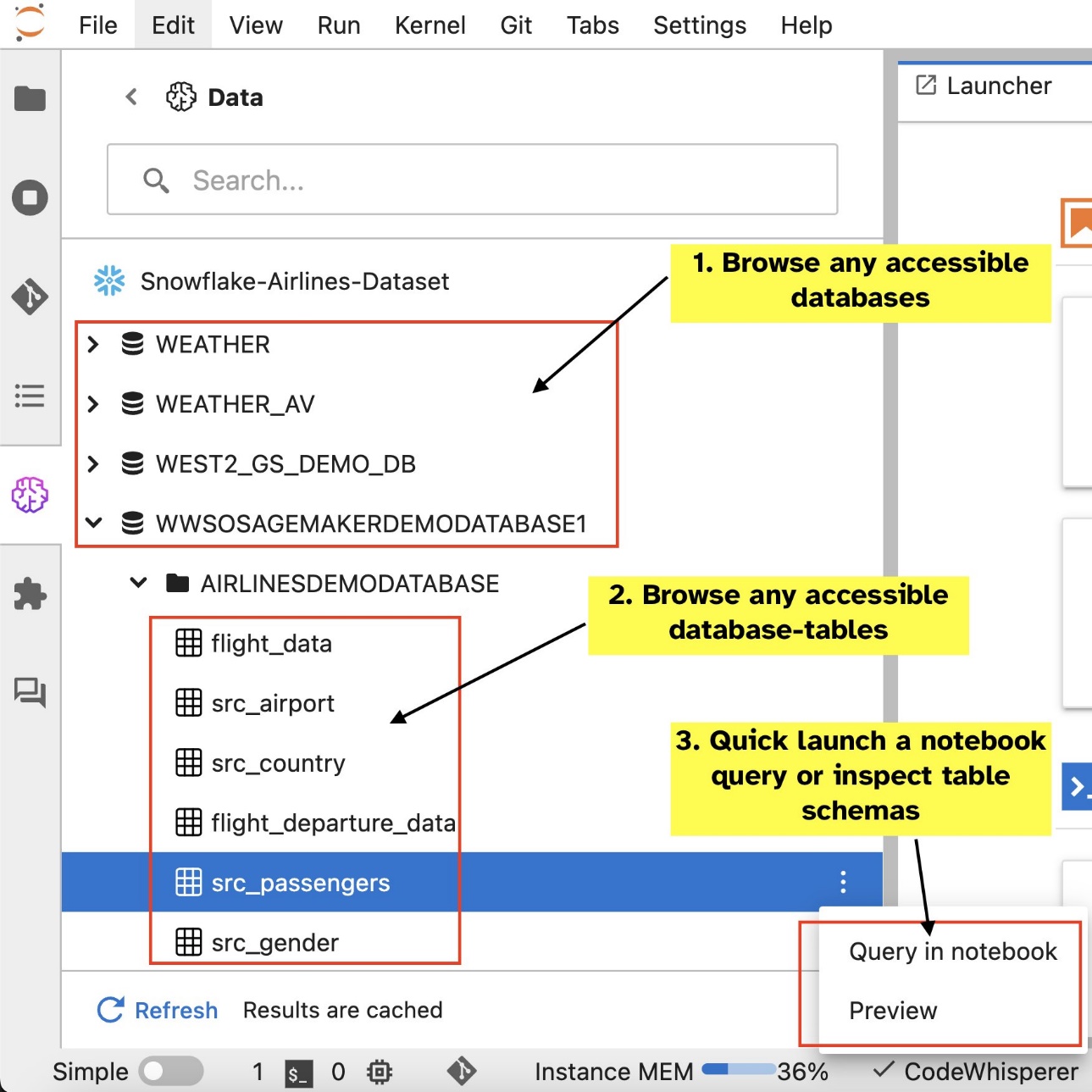
For example, you can visually explore data sources like databases, tables, and schemas directly from your JupyterLab ecosystem. If your notebook environments are running on SageMaker Distribution 1.6 or higher, look for a new widget on the left side of your JupyterLab interface. This addition enhances data accessibility and management within your development environment.
If you’re not currently on suggested SageMaker Distribution (1.5 or lower) or in a custom environment, refer to appendix for more information.
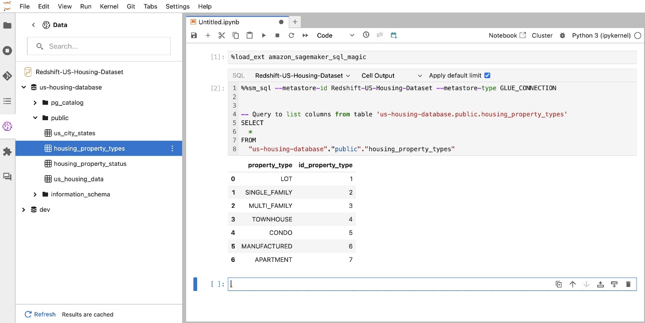
After you have set up connections (illustrated in the next section), you can list data connections, browse databases and tables, and inspect schemas.
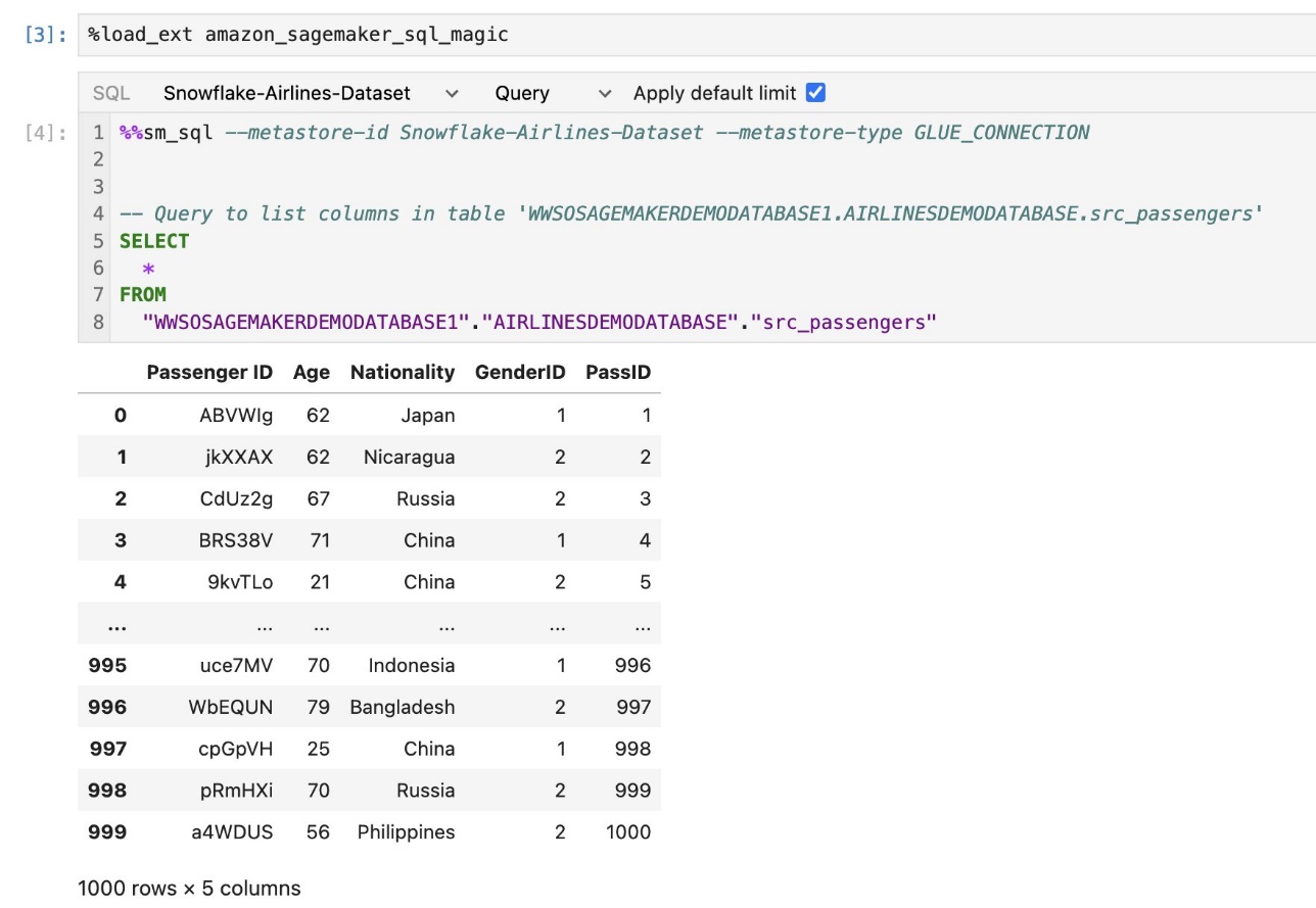
The SageMaker Studio JupyterLab built-in SQL extension also enables you to run SQL queries directly from a notebook. Jupyter notebooks can differentiate between SQL and Python code using the %%sm_sql magic command, which must be placed at the top of any cell that contains SQL code. This command signals to JupyterLab that the following instructions are SQL commands rather than Python code. The output of a query can be displayed directly within the notebook, facilitating seamless integration of SQL and Python workflows in your data analysis.
The output of a query can be displayed visually as HTML tables, as shown in the following screenshot.
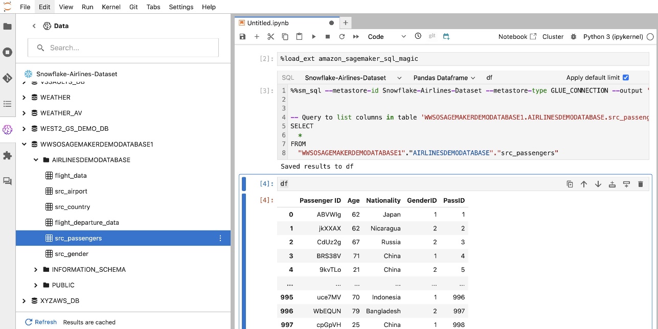
They can also be written to a pandas DataFrame.

Prerequisites
Make sure you have satisfied the following prerequisites in order to use the SageMaker Studio notebook SQL experience:
- SageMaker Studio V2 – Make sure you’re running the most up-to-date version of your SageMaker Studio domain and user profiles. If you’re currently on SageMaker Studio Classic, refer to Migrating from amazon SageMaker Studio Classic.
- IAM role – SageMaker requires an AWS Identity and Access Management (IAM) role to be assigned to a SageMaker Studio domain or user profile to manage permissions effectively. An execution role update may be required to bring in data browsing and the SQL run feature. The following example policy enables users to grant, list, and run AWS Glue, Athena, amazon Simple Storage Service (amazon S3), AWS Secrets Manager, and amazon Redshift resources:
- JupyterLab Space – You need access to the updated SageMaker Studio and JupyterLab Space with SageMaker Distribution v1.6 or later image versions. If you’re using custom images for JupyterLab Spaces or older versions of SageMaker Distribution (v1.5 or lower), refer to the appendix for instructions to install necessary packages and modules to enable this feature in your environments. To learn more about SageMaker Studio JupyterLab Spaces, refer to Boost productivity on amazon SageMaker Studio: Introducing JupyterLab Spaces and generative ai tools.
- Data source access credentials – This SageMaker Studio notebook feature requires user name and password access to data sources such as Snowflake and amazon Redshift. Create user name and password-based access to these data sources if you do not already have one. OAuth-based access to Snowflake is not a supported feature as of this writing.
- Load SQL magic – Before you run SQL queries from a Jupyter notebook cell, it’s essential to load the SQL magics extension. Use the command
%load_ext amazon_sagemaker_sql_magicto enable this feature. Additionally, you can run the%sm_sql?command to view a comprehensive list of supported options for querying from a SQL cell. These options include setting a default query limit of 1,000, running a full extraction, and injecting query parameters, among others. This setup allows for flexible and efficient SQL data manipulation directly within your notebook environment.
Create database connections
The built-in SQL browsing and execution capabilities of SageMaker Studio are enhanced by AWS Glue connections. An AWS Glue connection is an AWS Glue Data Catalog object that stores essential data such as login credentials, URI strings, and virtual private cloud (VPC) information for specific data stores. These connections are used by AWS Glue crawlers, jobs, and development endpoints to access various types of data stores. You can use these connections for both source and target data, and even reuse the same connection across multiple crawlers or extract, transform, and load (ETL) jobs.
To explore SQL data sources in the left pane of SageMaker Studio, you first need to create AWS Glue connection objects. These connections facilitate access to different data sources and allow you to explore their schematic data elements.
In the following sections, we walk through the process of creating SQL-specific AWS Glue connectors. This will enable you to access, view, and explore datasets across a variety of data stores. For more detailed information about AWS Glue connections, refer to Connecting to data.
Create an AWS Glue connection
The only way to bring data sources into SageMaker Studio is with AWS Glue connections. You need to create AWS Glue connections with specific connection types. As of this writing, the only supported mechanism of creating these connections is using the AWS Command Line Interface (AWS CLI).
Connection definition JSON file
When connecting to different data sources in AWS Glue, you must first create a JSON file that defines the connection properties—referred to as the connection definition file. This file is crucial for establishing an AWS Glue connection and should detail all the necessary configurations for accessing the data source. For security best practices, it’s recommended to use Secrets Manager to securely store sensitive information such as passwords. Meanwhile, other connection properties can be managed directly through AWS Glue connections. This approach makes sure that sensitive credentials are protected while still making the connection configuration accessible and manageable.
The following is an example of a connection definition JSON:
When setting up AWS Glue connections for your data sources, there are a few important guidelines to follow to provide both functionality and security:
- Stringification of properties – Within the
PythonPropertieskey, make sure all properties are stringified key-value pairs. It’s crucial to properly escape double-quotes by using the backslash (\) character where necessary. This helps maintain the correct format and avoid syntax errors in your JSON. - Handling sensitive information – Although it’s possible to include all connection properties within
PythonProperties, it is advisable not to include sensitive details like passwords directly in these properties. Instead, use Secrets Manager for handling sensitive information. This approach secures your sensitive data by storing it in a controlled and encrypted environment, away from the main configuration files.
Create an AWS Glue connection using the AWS CLI
After you include all the necessary fields in your connection definition JSON file, you’re ready to establish an AWS Glue connection for your data source using the AWS CLI and the following command:
This command initiates a new AWS Glue connection based on the specifications detailed in your JSON file. The following is a quick breakdown of the command components:
- –region <REGION> – This specifies the AWS Region where your AWS Glue connection will be created. It is crucial to select the Region where your data sources and other services are located to minimize latency and comply with data residency requirements.
- –cli-input-json file:///path/to/file/connection/definition/file.json – This parameter directs the AWS CLI to read the input configuration from a local file that contains your connection definition in JSON format.
You should be able to create AWS Glue connections with the preceding AWS CLI command from your Studio JupyterLab terminal. On the File menu, choose New and Terminal.
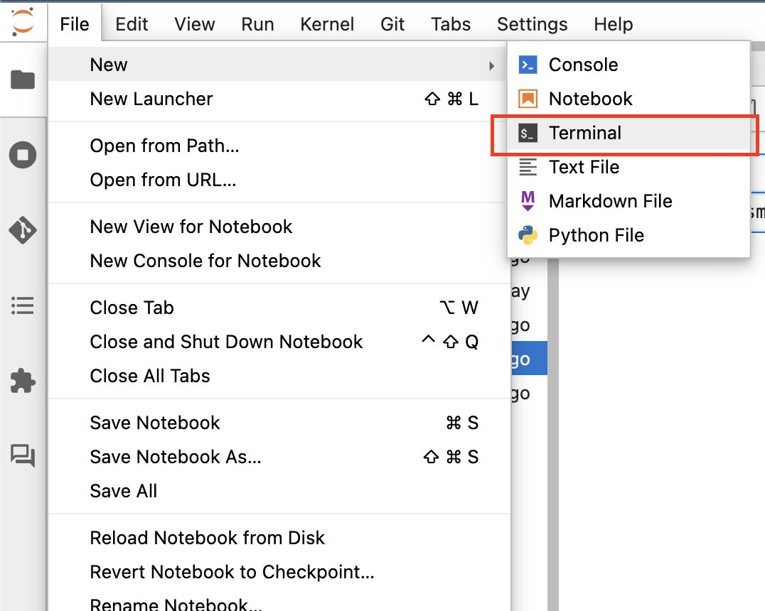
If the create-connection command runs successfully, you should see your data source listed in the SQL browser pane. If you don’t see your data source listed, choose Refresh to update the cache.

Create a Snowflake connection
In this section, we focus on integrating a Snowflake data source with SageMaker Studio. Creating Snowflake accounts, databases, and warehouses falls outside the scope of this post. To get started with Snowflake, refer to the Snowflake user guide. In this post, we concentrate on creating a Snowflake definition JSON file and establishing a Snowflake data source connection using AWS Glue.
Create a Secrets Manager secret
You can connect to your Snowflake account by either using a user ID and password or using private keys. To connect with a user ID and password, you need to securely store your credentials in Secrets Manager. As mentioned previously, although it’s possible to embed this information under PythonProperties, it is not recommended to store sensitive information in plain text format. Always make sure that sensitive data is handled securely to avoid potential security risks.
To store information in Secrets Manager, complete the following steps:
- On the Secrets Manager console, choose Store a new secret.
- For Secret type, choose Other type of secret.
- For the key-value pair, choose Plaintext and enter the following:
- Enter a name for your secret, such as
sm-sql-snowflake-secret. - Leave the other settings as default or customize if required.
- Create the secret.
Create an AWS Glue connection for Snowflake
As discussed earlier, AWS Glue connections are essential for accessing any connection from SageMaker Studio. You can find a list of all supported connection properties for Snowflake. The following is a sample connection definition JSON for Snowflake. Replace the placeholder values with the appropriate values before saving it to disk:
To create an AWS Glue connection object for the Snowflake data source, use the following command:
This command creates a new Snowflake data source connection in your SQL browser pane that’s browsable, and you can run SQL queries against it from your JupyterLab notebook cell.
Create an amazon Redshift connection
amazon Redshift is a fully managed, petabyte-scale data warehouse service that simplifies and reduces the cost of analyzing all your data using standard SQL. The procedure for creating an amazon Redshift connection closely mirrors that for a Snowflake connection.
Create a Secrets Manager secret
Similar to the Snowflake setup, to connect to amazon Redshift using a user ID and password, you need to securely store the secrets information in Secrets Manager. Complete the following steps:
- On the Secrets Manager console, choose Store a new secret.
- For Secret type, choose Credentials for amazon Redshift cluster.
- Enter the credentials used to log in to access amazon Redshift as a data source.
- Choose the Redshift cluster associated with the secrets.
- Enter a name for the secret, such as
sm-sql-redshift-secret. - Leave the other settings as default or customize if required.
- Create the secret.
By following these steps, you make sure your connection credentials are handled securely, using the robust security features of AWS to manage sensitive data effectively.
Create an AWS Glue connection for amazon Redshift
To set up a connection with amazon Redshift using a JSON definition, fill in the necessary fields and save the following JSON configuration to disk:
To create an AWS Glue connection object for the Redshift data source, use the following AWS CLI command:
This command creates a connection in AWS Glue linked to your Redshift data source. If the command runs successfully, you will be able to see your Redshift data source within the SageMaker Studio JupyterLab notebook, ready for running SQL queries and performing data analysis.
Create an Athena connection
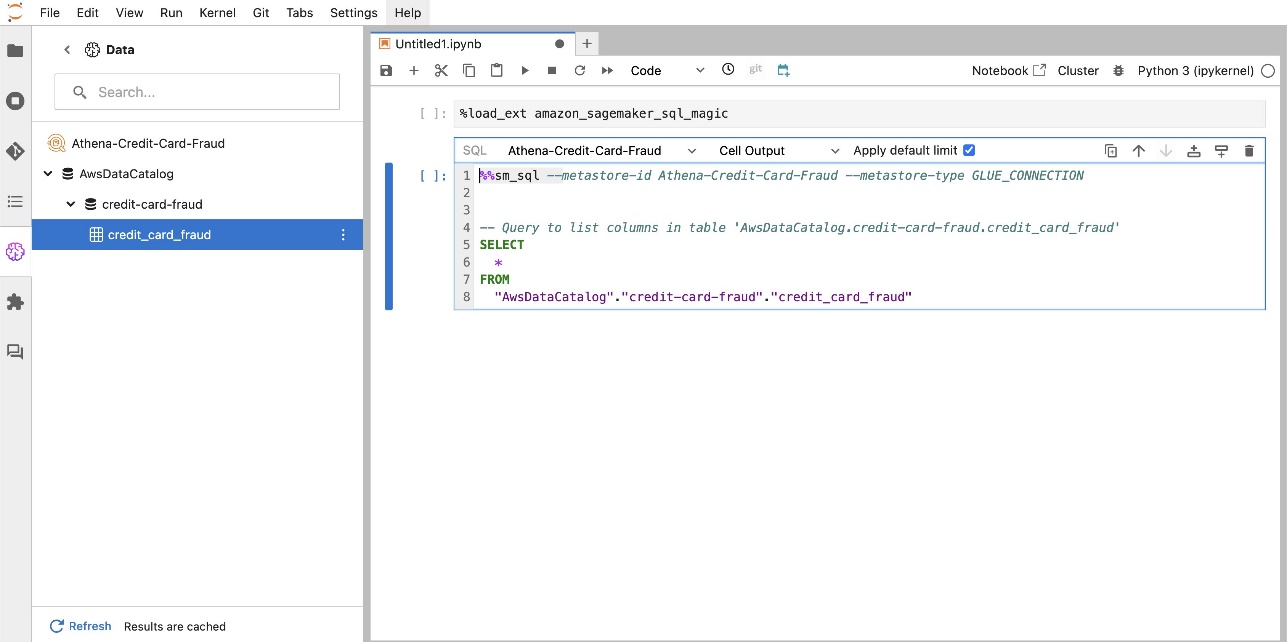
Athena is a fully managed SQL query service from AWS that enables analysis of data stored in amazon S3 using standard SQL. To set up an Athena connection as a data source in the JupyterLab notebook’s SQL browser, you need to create an Athena sample connection definition JSON. The following JSON structure configures the necessary details to connect to Athena, specifying the data catalog, the S3 staging directory, and the Region:
To create an AWS Glue connection object for the Athena data source, use the following AWS CLI command:
If the command is successful, you will be able to access Athena data catalog and tables directly from the SQL browser within your SageMaker Studio JupyterLab notebook.
Query data from multiple sources
If you have multiple data sources integrated into SageMaker Studio through the built-in SQL browser and the notebook SQL feature, you can quickly run queries and effortlessly switch between data source backends in subsequent cells within a notebook. This capability allows for seamless transitions between different databases or data sources during your analysis workflow.
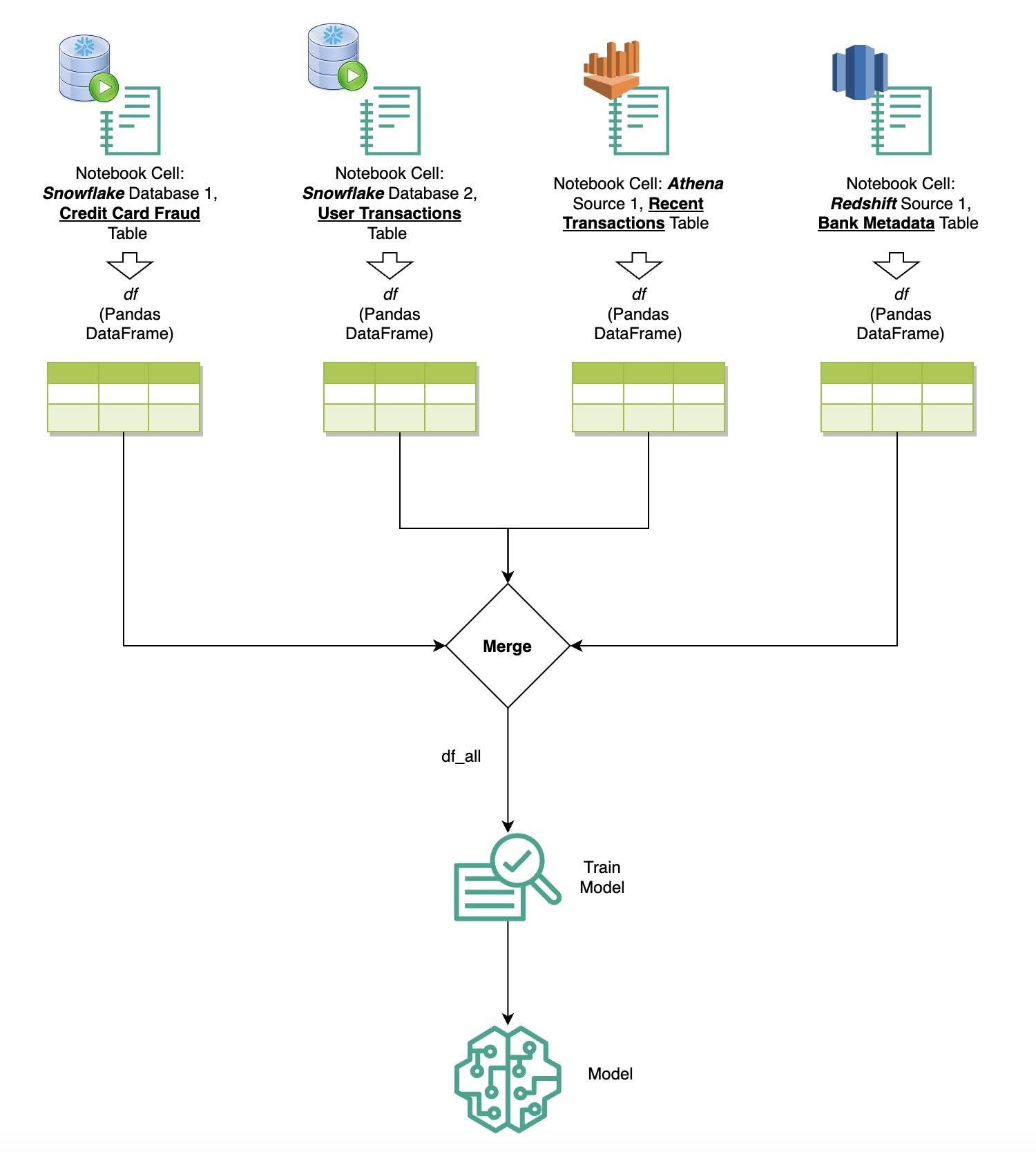
You can run queries against a diverse collection of data source backends and bring the results directly into the Python space for further analysis or visualization. This is facilitated by the %%sm_sql magic command available in SageMaker Studio notebooks. To output the results of your SQL query into a pandas DataFrame, there are two options:
- From your notebook cell toolbar, choose the output type DataFrame and name your DataFrame variable
- Append the following parameter to your
%%sm_sqlcommand:
The following diagram illustrates this workflow and showcases how you can effortlessly run queries across various sources in subsequent notebook cells, as well as train a SageMaker model using training jobs or directly within the notebook using local compute. Additionally, the diagram highlights how the built-in SQL integration of SageMaker Studio simplifies the processes of extraction and building directly within the familiar environment of a JupyterLab notebook cell.
Text to SQL: Using natural language to enhance query authoring
SQL is a complex language that requires an understanding of databases, tables, syntaxes, and metadata. Today, generative artificial intelligence (ai) can enable you to write complex SQL queries without requiring in-depth SQL experience. The advancement of LLMs has significantly impacted natural language processing (NLP)-based SQL generation, allowing for the creation of precise SQL queries from natural language descriptions—a technique referred to as Text-to-SQL. However, it is essential to acknowledge the inherent differences between human language and SQL. Human language can sometimes be ambiguous or imprecise, whereas SQL is structured, explicit, and unambiguous. Bridging this gap and accurately converting natural language into SQL queries can present a formidable challenge. When provided with appropriate prompts, LLMs can help bridge this gap by understanding the intent behind the human language and generating accurate SQL queries accordingly.
With the release of the SageMaker Studio in-notebook SQL query feature, SageMaker Studio makes it straightforward to inspect databases and schemas, and author, run, and debug SQL queries without ever leaving the Jupyter notebook IDE. This section explores how the Text-to-SQL capabilities of advanced LLMs can facilitate the generation of SQL queries using natural language within Jupyter notebooks. We employ the cutting-edge Text-to-SQL model defog/sqlcoder-7b-2 in conjunction with Jupyter ai, a generative ai assistant specifically designed for Jupyter notebooks, to create complex SQL queries from natural language. By using this advanced model, we can effortlessly and efficiently create complex SQL queries using natural language, thereby enhancing our SQL experience within notebooks.
Notebook prototyping using the Hugging Face Hub
To begin prototyping, you need the following:
- GitHub code – The code presented in this section is available in the following GitHub repo and by referencing the example notebook.
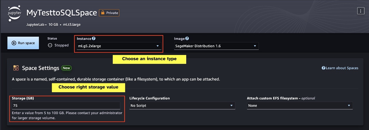
- JupyterLab Space – Access to a SageMaker Studio JupyterLab Space backed by GPU-based instances is essential. For the
defog/sqlcoder-7b-2model, a 7B parameter model, using an ml.g5.2xlarge instance is recommended. Alternatives such asdefog/sqlcoder-70b-alpha ordefog/sqlcoder-34b-alphaare also viable for natural language to SQL conversion, but larger instance types may be required for prototyping. Make sure you have the quota to launch a GPU-backed instance by navigating to the Service Quotas console, searching for SageMaker, and searching forStudio JupyterLab Apps running on <instance type>.

Launch a new GPU-backed JupyterLab Space from your SageMaker Studio. It’s recommended to create a new JupyterLab Space with at least 75 GB of amazon Elastic Block Store (amazon EBS) storage for a 7B parameter model.

- Hugging Face Hub – If your SageMaker Studio domain has access to download models from the Hugging Face Hub, you can use the
AutoModelForCausalLMclass from huggingface/transformers to automatically download models and pin them to your local GPUs. The model weights will be stored in your local machine’s cache. See the following code:
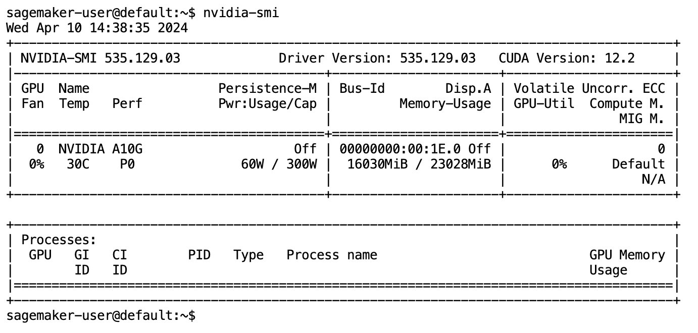
After the model has been fully downloaded and loaded into memory, you should observe an increase in GPU utilization on your local machine. This indicates that the model is actively using the GPU resources for computational tasks. You can verify this in your own JupyterLab space by running nvidia-smi (for a one-time display) or nvidia-smi —loop=1 (to repeat every second) from your JupyterLab terminal.
Text-to-SQL models excel at understanding the intent and context of a user’s request, even when the language used is conversational or ambiguous. The process involves translating natural language inputs into the correct database schema elements, such as table names, column names, and conditions. However, an off-the-shelf Text-to-SQL model will not inherently know the structure of your data warehouse, the specific database schemas, or be able to accurately interpret the content of a table based solely on column names. To effectively use these models to generate practical and efficient SQL queries from natural language, it is necessary to adapt the SQL text-generation model to your specific warehouse database schema. This adaptation is facilitated through the use of LLM prompts. The following is a recommended prompt template for the defog/sqlcoder-7b-2 Text-to-SQL model, divided into four parts:
- Task – This section should specify a high-level task to be accomplished by the model. It should include the type of database backend (such as amazon RDS, PostgreSQL, or amazon Redshift) to make the model aware of any nuanced syntactical differences that may affect the generation of the final SQL query.
- Instructions – This section should define task boundaries and domain awareness for the model, and may include few-shot examples to guide the model in generating finely tuned SQL queries.
- Database Schema – This section should detail your warehouse database schemas, outlining the relationships between tables and columns to aid the model in understanding the database structure.
- Answer – This section is reserved for the model to output the SQL query response to the natural language input.
An example of the database schema and prompt used in this section is available in the GitHub Repo.
Prompt engineering is not just about forming questions or statements; it’s a nuanced art and science that significantly impacts the quality of interactions with an ai model. The way you craft a prompt can profoundly influence the nature and usefulness of the ai’s response. This skill is pivotal in maximizing the potential of ai interactions, especially in complex tasks requiring specialized understanding and detailed responses.
It’s important to have the option to quickly build and test a model’s response for a given prompt and optimize the prompt based on the response. JupyterLab notebooks provide the ability to receive instant model feedback from a model running on local compute and optimize the prompt and tune a model’s response further or change a model entirely. In this post, we use a SageMaker Studio JupyterLab notebook backed by ml.g5.2xlarge’s NVIDIA A10G 24 GB GPU to run Text-to-SQL model inference on the notebook and interactively build our model prompt until the model’s response is sufficiently tuned to provide responses that are directly executable in JupyterLab’s SQL cells. To run model inference and simultaneously stream model responses, we use a combination of model.generate and TextIteratorStreamer as defined in the following code:
The model’s output can be decorated with SageMaker SQL magic %%sm_sql ..., which allows the JupyterLab notebook to identify the cell as a SQL cell.
Host Text-to-SQL models as SageMaker endpoints
At the end of the prototyping stage, we have selected our preferred Text-to-SQL LLM, an effective prompt format, and an appropriate instance type for hosting the model (either single-GPU or multi-GPU). SageMaker facilitates the scalable hosting of custom models through the use of SageMaker endpoints. These endpoints can be defined according to specific criteria, allowing for the deployment of LLMs as endpoints. This capability enables you to scale the solution to a wider audience, allowing users to generate SQL queries from natural language inputs using custom hosted LLMs. The following diagram illustrates this architecture.

To host your LLM as a SageMaker endpoint, you generate several artifacts.
The first artifact is model weights. SageMaker Deep Java Library (DJL) Serving containers allow you to set up configurations through a meta serving.properties file, which enables you to direct how models are sourced—either directly from the Hugging Face Hub or by downloading model artifacts from amazon S3. If you specify model_id=defog/sqlcoder-7b-2, DJL Serving will attempt to directly download this model from the Hugging Face Hub. However, you may incur networking ingress/egress charges each time the endpoint is deployed or elastically scaled. To avoid these charges and potentially speed up the download of model artifacts, it is recommended to skip using model_id in serving.properties and save model weights as S3 artifacts and only specify them with s3url=s3://path/to/model/bin.
Saving a model (with its tokenizer) to disk and uploading it to amazon S3 can be accomplished with just a few lines of code:
You also use a database prompt file. In this setup, the database prompt is composed of Task, Instructions, Database Schema, and Answer sections. For the current architecture, we allocate a separate prompt file for each database schema. However, there is flexibility to expand this setup to include multiple databases per prompt file, allowing the model to run composite joins across databases on the same server. During our prototyping stage, we save the database prompt as a text file named <Database-Glue-Connection-Name>.prompt, where Database-Glue-Connection-Name corresponds to the connection name visible in your JupyterLab environment. For instance, this post refers to a Snowflake connection named Airlines_Dataset, so the database prompt file is named Airlines_Dataset.prompt. This file is then stored on amazon S3 and subsequently read and cached by our model serving logic.
Moreover, this architecture permits any authorized users of this endpoint to define, store, and generate natural language to SQL queries without the need for multiple redeployments of the model. We use the following example of a database prompt to demonstrate the Text-to-SQL functionality.
Next, you generate custom model service logic. In this section, you outline a custom inference logic named model.py. This script is designed to optimize the performance and integration of our Text-to-SQL services:
- Define the database prompt file caching logic – To minimize latency, we implement a custom logic for downloading and caching database prompt files. This mechanism makes sure that prompts are readily available, reducing the overhead associated with frequent downloads.
- Define custom model inference logic – To enhance inference speed, our text-to-SQL model is loaded in the float16 precision format and then converted into a DeepSpeed model. This step allows for more efficient computation. Additionally, within this logic, you specify which parameters users can adjust during inference calls to tailor the functionality according to their needs.
- Define custom input and output logic – Establishing clear and customized input/output formats is essential for smooth integration with downstream applications. One such application is JupyterAI, which we discuss in the subsequent section.
Additionally, we include a serving.properties file, which acts as a global configuration file for models hosted using DJL serving. For more information, refer to Configurations and settings.
Lastly, you can also include a requirements.txt file to define additional modules required for inference and package everything into a tarball for deployment.
See the following code:
Integrate your endpoint with the SageMaker Studio Jupyter ai assistant
ai.readthedocs.io/en/latest/” target=”_blank” rel=”noopener”>Jupyter ai is an open source tool that brings generative ai to Jupyter notebooks, offering a robust and user-friendly platform for exploring generative ai models. It enhances productivity in JupyterLab and Jupyter notebooks by providing features like the %%ai magic for creating a generative ai playground inside notebooks, a native chat UI in JupyterLab for interacting with ai as a conversational assistant, and support for a wide array of LLMs from providers like amazon Titan, AI21, Anthropic, Cohere, and Hugging Face or managed services like amazon Bedrock and SageMaker endpoints. For this post, we use Jupyter ai’s out-of-the-box integration with SageMaker endpoints to bring the Text-to-SQL capability into JupyterLab notebooks. The Jupyter ai tool comes pre-installed in all SageMaker Studio JupyterLab Spaces backed by SageMaker Distribution images; end-users are not required to make any additional configurations to start using the Jupyter ai extension to integrate with a SageMaker hosted endpoint. In this section, we discuss the two ways to use the integrated Jupyter ai tool.
Jupyter ai inside a notebook using magics
Jupyter ai’s %%ai magic command allows you to transform your SageMaker Studio JupyterLab notebooks into a reproducible generative ai environment. To begin using ai magics, make sure you have loaded the jupyter_ai_magics extension to use %%ai magic, and additionally load amazon_sagemaker_sql_magic to use %%sm_sql magic:
To run a call to your SageMaker endpoint from your notebook using the %%ai magic command, provide the following parameters and structure the command as follows:
- –region-name – Specify the Region where your endpoint is deployed. This makes sure that the request is routed to the correct geographic location.
- –request-schema – Include the schema of the input data. This schema outlines the expected format and types of the input data that your model needs to process the request.
- –response-path – Define the path within the response object where the output of your model is located. This path is used to extract the relevant data from the response returned by your model.
- -f (optional) – This is an ai.readthedocs.io/en/latest/users/index.html#formatting-the-output” target=”_blank” rel=”noopener”>output formatter flag that indicates the type of output returned by the model. In the context of a Jupyter notebook, if the output is code, this flag should be set accordingly to format the output as executable code at the top of a Jupyter notebook cell, followed by a free text input area for user interaction.
For example, the command in a Jupyter notebook cell might look like the following code:
Jupyter ai chat window
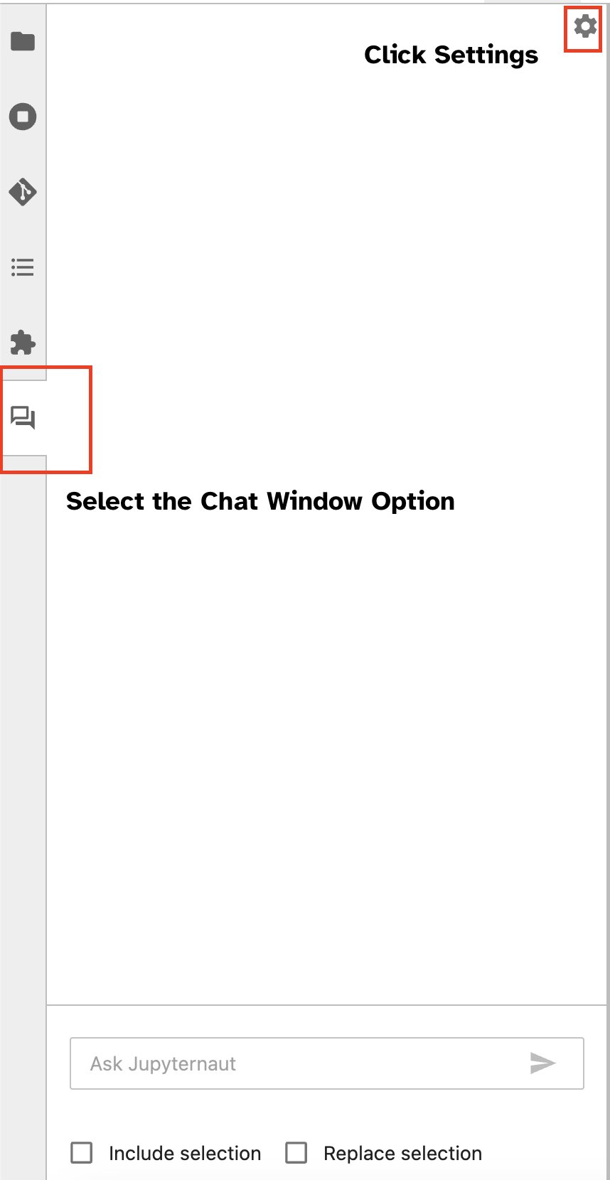
Alternatively, you can interact with SageMaker endpoints through a built-in user interface, simplifying the process of generating queries or engaging in dialogue. Before beginning to chat with your SageMaker endpoint, configure the relevant settings in Jupyter ai for the SageMaker endpoint, as shown in the following screenshot.
 |
 |
Conclusion
SageMaker Studio now simplifies and streamlines the data scientist workflow by integrating SQL support into JupyterLab notebooks. This allows data scientists to focus on their tasks without the need to manage multiple tools. Furthermore, the new built-in SQL integration in SageMaker Studio enables data personas to effortlessly generate SQL queries using natural language text as input, thereby accelerating their workflow.
We encourage you to explore these features in SageMaker Studio. For more information, refer to Prepare data with SQL in Studio.
Appendix
Enable the SQL browser and notebook SQL cell in custom environments
If you’re not using a SageMaker Distribution image or using Distribution images 1.5 or below, run the following commands to enable the SQL browsing feature inside your JupyterLab environment:
Relocate the SQL browser widget
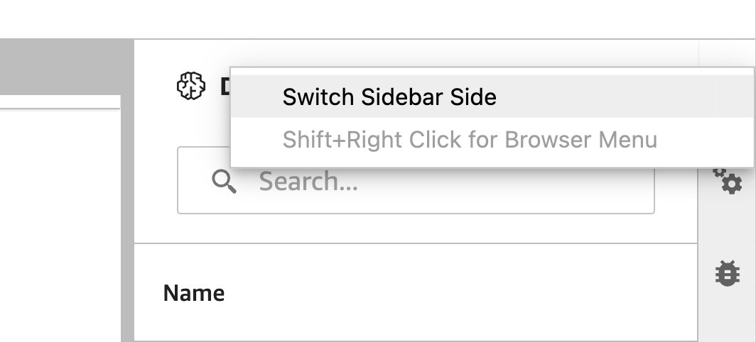
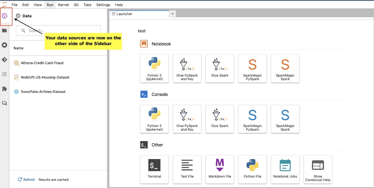
JupyterLab widgets allow for relocation. Depending on your preference, you can move widgets to the either side of JupyterLab widgets pane. If you prefer, you can move the direction of the SQL widget to the opposite side (right to left) of the sidebar with a simple right-click on the widget icon and choosing Switch Sidebar Side.
 |
 |
About the authors
 Pranav Murthy is an ai/ML Specialist Solutions Architect at AWS. He focuses on helping customers build, train, deploy and migrate machine learning (ML) workloads to SageMaker. He previously worked in the semiconductor industry developing large computer vision (CV) and natural language processing (NLP) models to improve semiconductor processes using state of the art ML techniques. In his free time, he enjoys playing chess and traveling. You can find Pranav on LinkedIn.
 Varun Shah is a Software Engineer working on amazon SageMaker Studio at amazon Web Services. He is focused on building interactive ML solutions which simplify data processing and data preparation journeys . In his spare time, Varun enjoys outdoor activities including hiking and skiing, and is always up for discovering new, exciting places.
 Sumedha Swamy is a Principal Product Manager at amazon Web Services where he leads SageMaker Studio team in its mission to develop IDE of choice for data science and machine learning. He has dedicated the past 15 years building Machine Learning based consumer and enterprise products.
 Bosco Albuquerque is a Sr. Partner Solutions Architect at AWS and has over 20 years of experience working with database and analytics products from enterprise database vendors and cloud providers. He has helped technology companies design and implement data analytics solutions and products.
 NEWSLETTER


