Introduction
Activation functions are the secret sauce behind the remarkable capabilities of neural networks. They are the decision-makers, determining whether a neuron should “fire up” or remain dormant based on the input it receives. While this might sound like an intricate technicality, understanding activation functions is crucial for anyone diving into artificial neural networks.
In this blog post, we’ll demystify activation functions in a way that’s easy to grasp, even if you’re new to machine learning. Think of it as the key to unlocking the hidden potential of neural networks. By the end of this article, you’ll comprehend what activation functions are and appreciate their significance in deep learning.
So, whether you’re a budding data scientist, a machine learning enthusiast, or simply curious about the magic happening inside those neural networks, fasten your seatbelt. Let’s embark on a journey to explore the heart of artificial intelligence: activation functions.
Learning Objectives
- Understand activation functions’ role and transformation in neural networks.
- Explore commonly used activation functions and their pros and cons.
- Recognize scenarios for specific activation functions and their impact on gradient flow.
This article was published as a part of the Data Science Blogathon.
What is the Activation Function?
Activation functions are the decision-makers within a neural network. They are attached to each neuron and play a pivotal role in determining whether a neuron should be activated. This activation decision hinges on whether the input received by each neuron is relevant to the network’s prediction.
Activation functions act as gatekeepers, allowing only certain information to pass through and contribute to the network’s output. They add an essential layer of non-linearity to neural networks, enabling them to learn and represent complex patterns within data.
To dive deeper into this crucial concept, explore some standard activation functions and their unique characteristics. The activation function also plays a vital role in normalizing each neuron’s output, constraining it within a specific range, typically between 0 and 1 or between -1 and 1.
In a neural network, inputs are supplied to the neurons within the input layer. Each neuron is associated with a weight, and the output of the neuron is calculated by multiplying the input with its respective weight. This output is then passed on to the next layer.
The activation function is a mathematical ‘gate’ between the input entering the current neuron and the output transmitted to the subsequent layer. It can be as straightforward as a step function, effectively switching the neuron output on or off based on a defined rule or threshold.
Crucially, neural networks employ non-linear activation functions. These functions are instrumental in enabling the network to understand intricate data patterns, compute and learn nearly any function relevant to a given question, and ultimately make precise predictions.
Learn More: Activation Functions | Fundamentals Of Deep Learning
Commonly Used Activation Functions
- Sigmoid function
- tanh function
- ReLU function
- Leaky ReLU function
- ELU (Exponential Linear Units) function
Sigmoid Function
The sigmoid function formula and curve are as follows,

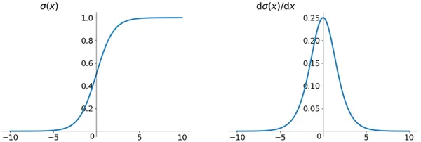
The Sigmoid function is the most frequently used activation function at the beginning of deep learning. It is a smoothing function that is easy to derive.
The sigmoid function shows its output is in the open interval (0,1). We can think of probability, but in the strict sense, don’t treat it as a probability. The sigmoid function was once more widespread. It can be thought of as the firing rate of a neuron. In the middle, where the slope is relatively large, it is the sensitive area of the neuron. The neuron’s inhibitory area is on the sides, with a gentle slope.
Think of the Sigmoid function as a way to describe how active or “fired up” a neuron in a neural network is. Imagine you have a neuron, like a switch, in your network.
- When the Sigmoid function’s output is close to 1, you can picture the neuron as highly sensitive, like it’s ready to respond strongly to input.
- In the middle, where the slope is steep, this is where the neuron is most sensitive. If you change the input slightly, the neuron’s output will change significantly.
- On the sides where the slope is gentle, it’s like the neuron is in an inhibitory area. Here, even if you change the input slightly, the neuron doesn’t react much. It’s not very sensitive in these areas.
The function itself has certain defects.
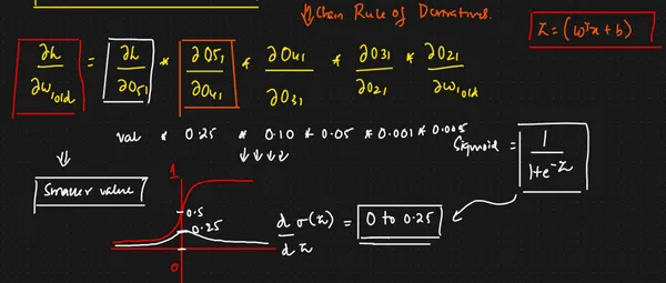
- When the input is slightly away from the coordinate origin, the function’s gradient becomes very small, almost zero.
- Why are values zero or negligible?
- The sigmoid Function output interval is 0 or 1. The formula of the sigmoid function is F(x) = 1 / (1 + e^-z), so we put the value z = 0 or 1. (1 + e^-z) is always higher. but this term is present on the denominator, so the overall calculation is very small.
- So, gradient function values are very small or almost zero.
- In backpropagation in a neural network, we rely on the chain rule of differentiation to calculate the gradients of each weight (w). However, when backpropagation passes through the sigmoid function, the gradient in this chain can become extremely small. Moreover, if this occurs across multiple layers with sigmoid functions, it can lead to the weight (w) having minimal impact on the loss function. This situation isn’t favorable for weight optimization and is commonly called ‘gradient saturation’ or ‘gradient vanishing.’
- Consider a layer…

2. The function output is not centered on 0, which can reduce the efficiency of the weight update.
3. The sigmoid function involves exponential operations, which can be computationally slower for computers.
Advantages and Disadvantages of Signoid Function
| Advantages of Sigmoid Function | Disadvantages of Sigmoid Function |
|---|---|
| 1. Smooth Gradient: Helps prevent sudden jumps in output values during training. | 1. Prone to Gradient Vanishing: Especially in deep networks, which can hinder training. |
| 2. Output Bounded between 0 and 1: Normalizes neuron output. | 2. Function Output, not Zero-Centered: Activations may be positive or negative. |
| 3. Clear Predictions: Useful for binary decisions. | 3. Power Operations are Time-Consuming: Involves computationally expensive operations. |
Tanh Function
The tanh function formula and curve are as follows,

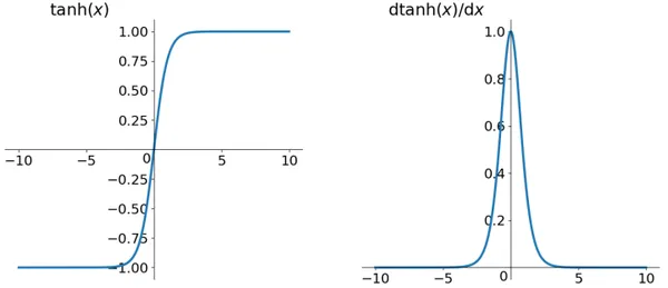
Tanh, short for hyperbolic tangent, is an activation function closely related to the sigmoid function. While the tanh and sigmoid function curves share similarities, there are noteworthy differences. Let’s compare them.
One common characteristic is that both functions produce nearly smooth outputs with small gradients when the input values are either very large or very small. This can pose challenges for efficient weight updates during training. However, the key distinction lies in their output intervals.
Tanh’s output interval ranges from -1 to 1, and the entire function is zero-centered, which sets it apart from the sigmoid function.
In many scenarios, the tanh function finds its place in the hidden layers of neural networks. In contrast, the sigmoid function is often employed in the output layer, especially in binary classification tasks. However, these choices are not set in stone and should be tailored to the specific problem or determined through experimentation and tuning.
Advantages and Disadvantages of Tanh Function
| Advantages of Tanh Function | Disadvantages of Tanh Function |
|---|---|
| 1. Zero-Centred Output: Outputs are centered around zero, aiding weight updates. | 1. Gradient Vanishing: Can suffer from gradient vanishing in deep networks. |
| 2. Smooth Gradient: Provides a smooth gradient, ensuring stable optimization. | 2. Computationally Intensive: Involves exponentials, potentially slower on large networks. |
| 3. Wider Output Range: A broader output range (-1 to 1) for capturing varied information. | 3. Output Not in (0, 1): Doesn’t bound output between 0 and 1, limiting specific applications. |
ReLU Function
The ReLU function formula and curve are as follows,


The ReLU function, short for Rectified Linear Unit, is a relatively recent and highly influential activation function in deep learning. Unlike some other activation functions, ReLU is remarkably straightforward. It simply outputs the maximum value between zero and its input. Although ReLU lacks full differentiability, we can employ a sub-gradient approach to handle its derivative, as illustrated in the figure above.
ReLU has gained widespread popularity in recent years, and for good reason. It stands out compared to traditional activation functions like the sigmoid and tanh.
Advantages and Disadvantages of ReLU Function
| Advantages of ReLU Function | Disadvantages of ReLU Function |
|---|---|
| 1. Simplicity: Easy to implement and efficient. | 1. Dead Neurons: Negative inputs can lead to a ‘dying ReLU’ problem. |
| 2. Mitigation of Vanishing Gradient: Addresses vanishing gradient issue. | 2. Not Zero-Centered: Non-zero-centered function. |
| 3. Sparsity: Induces sparsity in activations. | 3. Sensitivity to Initialization: Requires careful weight initialization. |
| 4. Biological Inspiration: Mimics real neuron activation patterns. | 4. Not Suitable for All Tasks: It may not fit all problem types. |
| 5. Gradient Saturation Mitigation: No gradient saturation for positive inputs. | |
| 6. Computational Speed: Faster calculations compared to some functions. |
Leaky ReLU Function
The leaky ReLU function formula and curve are as follows,

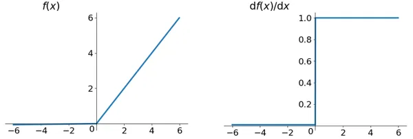
To address the ‘Dead ReLU Problem,’ researchers have proposed several solutions. One intuitive approach is to set the first half of ReLU to a small positive value like 0.01x instead of a strict 0. Another method, Parametric ReLU, introduces a learnable parameter, alpha. The Parametric ReLU function is f(x) = max(alpha * x, x). Through backpropagation, the network can determine the optimal value of alpha.(For selecting an alpha value, pick up the smallest value).
In theory, Leaky ReLU offers all the advantages of ReLU while eliminating the issues associated with ‘Dead ReLU.’ Leaky ReLU allows a small, non-zero gradient for negative inputs, preventing neurons from becoming inactive. However, whether Leaky ReLU consistently outperforms ReLU depends on the specific problem and architecture. There’s no one-size-fits-all answer, and the choice between ReLU and its variants often requires empirical testing and fine-tuning.
These variations of the ReLU function demonstrate the ongoing quest to enhance the performance and robustness of neural networks, catering to a wide range of applications and challenges in deep learning
Advantages and Disadvantages of Leaky ReLU Function
| Advantages of Leaky ReLU Function | Disadvantages of Leaky ReLU Function |
|---|---|
| 1. Mitigation of Dead Neurons: Prevents the ‘Dead ReLU’ issue by allowing a small gradient for negatives. | 1. Lack of Universality: May not be superior in all cases. |
| 2. Gradient Saturation Mitigation: Avoids gradient saturation for positive inputs. | 2. Additional Hyperparameter: Requires tuning of the ‘leakiness’ parameter. |
| 3. Simple Implementation: Easy to implement and computationally efficient. | 3. Not Zero-Centered: Non-zero-centered function. |
ELU (Exponential Linear Units) Function
ELU function formula and curve are as follows,

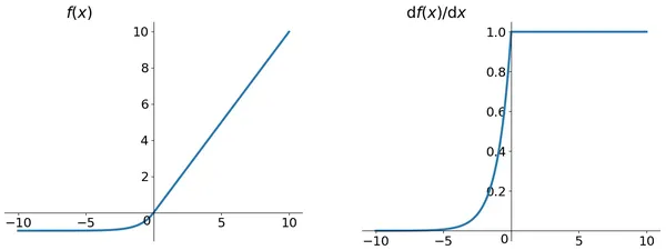
It is another activation function proposed to address some of the challenges posed by ReLU.
Advantages and Disadvantages of ELU Function
| Advantages of ELU Function | Disadvantages of ELU Function |
|---|---|
| 1. No Dead ReLU Issues: Eliminates the ‘Dead ReLU’ problem by allowing a small gradient for negatives. | 1. Computational Intensity: Slightly more computationally intensive due to exponentials. |
| 2. Zero-Centred Output: Outputs are zero-centered, facilitating specific optimization algorithms. | |
| 3. Smoothness: Smooth function across all input ranges. | |
| 4. Theoretical Advantages: Offers theoretical benefits over ReLU. |
Training Neural Networks with Activation Functions
The choice of activation functions in neural networks significantly impacts the training process. Activation functions are crucial in determining how neural networks learn and whether they can effectively model complex relationships within the data. Here, we’ll discuss how activation functions influence training, address issues like vanishing gradients, and how certain activation functions mitigate these challenges.
Impact of Activation Functions on Training:
- Activation functions determine how neurons transform input signals into output activations during forward propagation.
- During backpropagation, gradients calculated for each layer depend on the derivative of the activation function.
- The choice of activation function affects the overall training speed, stability, and convergence of neural networks.
Vanishing Gradients:
- Vanishing gradients occur when the derivatives of activation functions become extremely small, causing slow convergence or stagnation in training.
- Sigmoid and tanh activation functions are known for causing vanishing gradients, especially in deep networks.
Mitigating the Vanishing Gradient Problem:
- Rectified Linear Unit (ReLU) and its variants, such as Leaky ReLU, address the vanishing gradient problem by providing a non-zero gradient for positive inputs.
- ReLU functions result in faster convergence due to the lack of vanishing gradients when inputs are positive.
Role of Zero-Centered Activation Functions:
- Activation functions like ELU, which offer zero-centered output, help mitigate the vanishing gradient problem by providing both positive and negative gradients.
- Zero-centered functions contribute to stable weight updates and optimization during training.
Adaptive Activation Choices:
- The choice of activation function should align with the network’s architecture and the specific problem’s requirements.
- It’s essential to empirically test different activation functions to determine the most suitable one for a given task.
Practical Examples
Using TensorFlow and Keras
import tensorflow as tf
from tensorflow.keras.layers import Dense
from tensorflow.keras.models import Sequential

# Sample data
x = ((-1.0, 0.0, 1.0), (-2.0, 2.0, 3.0))

# Sigmoid activation
model_sigmoid = Sequential((Dense(3, activation='sigmoid', input_shape=(3,))))
output_sigmoid = model_sigmoid.predict(x)

# Tanh activation
model_tanh = Sequential((Dense(3, activation='tanh', input_shape=(3,))))
output_tanh = model_tanh.predict(x)

# ReLU activation
model_relu = Sequential((Dense(3, activation='relu', input_shape=(3,))))
output_relu = model_relu.predict(x)

# Leaky ReLU activation
model_leaky_relu = Sequential((Dense(3, activation=tf.nn.leaky_relu, input_shape=(3,))))
output_leaky_relu = model_leaky_relu.predict(x)

# ELU activation
model_elu = Sequential((Dense(3, activation='elu', input_shape=(3,))))
output_elu = model_elu.predict(x)

print("Sigmoid Output:\n", output_sigmoid)
print("Tanh Output:\n", output_tanh)
print("ReLU Output:\n", output_relu)
print("Leaky ReLU Output:\n", output_leaky_relu)
print("ELU Output:\n", output_elu)
#import csv
Using PyTorch
import torch
import torch.nn as nn

# Sample data
x = torch.tensor(((-1.0, 0.0, 1.0), (-2.0, 2.0, 3.0)), dtype=torch.float32)

# Sigmoid activation
sigmoid = nn.Sigmoid()
output_sigmoid = sigmoid(x)

# Tanh activation
tanh = nn.Tanh()
output_tanh = tanh(x)

# ReLU activation
relu = nn.ReLU()
output_relu = relu(x)

# Leaky ReLU activation
leaky_relu = nn.LeakyReLU(negative_slope=0.01)
output_leaky_relu = leaky_relu(x)

# ELU activation
elu = nn.ELU()
output_elu = elu(x)

print("Sigmoid Output:\n", output_sigmoid)
print("Tanh Output:\n", output_tanh)
print("ReLU Output:\n", output_relu)
print("Leaky ReLU Output:\n", output_leaky_relu)
print("ELU Output:\n", output_elu)
Here are the outputs for the provided code examples using different activation functions:
Sigmoid Output:
Sigmoid Output:
 ((0.26894143  0.5        0.7310586 )
 ( 0.11920292  0.8807971  0.95257413))
Tanh Output:
Tanh Output:
 ((-0.7615942  0.         0.7615942)
 (-0.9640276   0.9640276  0.9950547))
ReLU Output:
ReLU Output:
 ((0. 2. 3.)
 ( 0. 2. 3.))
Leaky ReLU Output:
Leaky ReLU Output:
 ((-0.01  0.    1.  )
 (-0.02   2.    3.  ))
ELU Output:
ELU Output:
 ((-0.63212055   0.   1. )
 (-1.2642411     2.   3. ))
Conclusion
Activation functions are the lifeblood of neural networks, dictating how these computational systems process information. From the classic Sigmoid and Tanh to the efficiency of ReLU and its variants, we’ve explored their roles in shaping neural network behavior. Each function offers unique strengths and weaknesses, and choosing the right one depends on the nature of your data and the specific problem you’re tackling. With practical implementation insights, you’re now equipped to make informed decisions, harnessing these functions to optimize your neural network’s performance and unlock the potential of deep learning in your projects.
Key Takeaways:
- Activation functions are fundamental in neural networks, transforming input signals and enabling the learning of complex data relationships.
- Common activation functions include Sigmoid, Tanh, ReLU, Leaky ReLU, and ELU, each with unique characteristics and use cases.
- Understanding the advantages and disadvantages of activation functions helps select the most suitable one for specific neural network tasks.
- Activation functions are critical in addressing gradient issues, such as gradient vanishing, during backpropagation.
Frequently Asked Questions (FAQs)
A. An activation function is a mathematical operation applied to the output of a neuron in a neural network, introducing non-linearity and enabling the network to learn complex patterns.
A. ReLU offers simplicity, faster convergence in deep networks, and computational efficiency. It’s widely used for its benefits in training.
A. The choice of activation function depends on factors like data nature, network architecture, and specific problems. Different functions have strengths suited to different scenarios.
A. Yes, certain activation functions are more suitable for specific tasks. For example, Sigmoid and Tanh are commonly used in binary classification, while ReLU is favored in deep learning tasks like image recognition.
A. Activation functions are crucial in gradient flow during backpropagation, influencing training speed and overall network performance. The right choice can improve convergence and model effectiveness.
The media shown in this article is not owned by Analytics Vidhya and is used at the Author’s discretion.


