Building Efficient Neural Networks with JAX

Flax is an advanced neural network library built on top of JAX, aimed at giving researchers and developers a flexible, high-performance toolset for building complex machine learning models. Flax’s seamless integration with JAX enables automatic differentiation, Just-In-Time (JIT) compilation, and support for hardware accelerators, making it ideal for both experimental research and production.

This blog will explore Flax’s core features, compare them to other frameworks, and provide a practical example using Flax’s functional programming approach.

Learning Objective

• Understand Flax as a high-performance, flexible neural network library built on JAX suitable for research and production.
• Learn how Flax’s functional programming approach improves the reproducibility and debugging of machine-learning models.
• Explore Flax’s Linen API for efficiently building and managing complex neural network architectures.
• Discover the integration of Flax with Optax for streamlined optimization and gradient processing in training workflows.
• Gain insights into Flax’s parameter management, state handling, and model serialization for better deployment and persistence.

This article was published as a part of the Data Science Blogathon.

What is Flax?

Flax is a high-performance neural network library built on top of JAX, designed to provide researchers and developers with the flexibility and efficiency needed to build cutting-edge machine learning models. Flax leverages JAX’s capabilities, such as automatic differentiation and Just-In-Time (JIT) compilation, to offer a powerful framework for both research and production environments.

The Comparison: Flax vs. Other Frameworks

Flax distinguishes itself from other deep learning frameworks like TensorFlow, PyTorch, and Keras through its unique design principles:

• Functional Programming Paradigm: Flax embraces a purely functional style, treating models as pure functions without hidden states. This approach enhances reproducibility and ease of debugging.
• Composability with JAX: By leveraging JAX’s transformations (jit, grad, vmap), Flax allows for seamless optimization and parallelization of model computations.
• Modularity: Flax’s module system promotes the construction of reusable components, making it easier to construct complex architectures from simple building blocks.
• Performance: Built on JAX, Flax inherits its high-performance capabilities, including support for hardware accelerators like GPUs and TPUs.

Key Features of Flax

• Linen API: Flax’s high-level API for defining neural network layers and models emphasises clarity and ease of use.
• Parameter Management: Efficient handling of model parameters using immutable data structures, promoting functional purity.
• Integration with Optax: Seamless compatibility with Optax, a gradient processing and optimization library for JAX.
• Serialization: Robust tools for saving and loading model parameters, facilitating model persistence and deployment.
• Extensibility: Ability to create custom modules and integrate them with other JAX-based libraries.

Also read: Flax

Setting Up the Environment

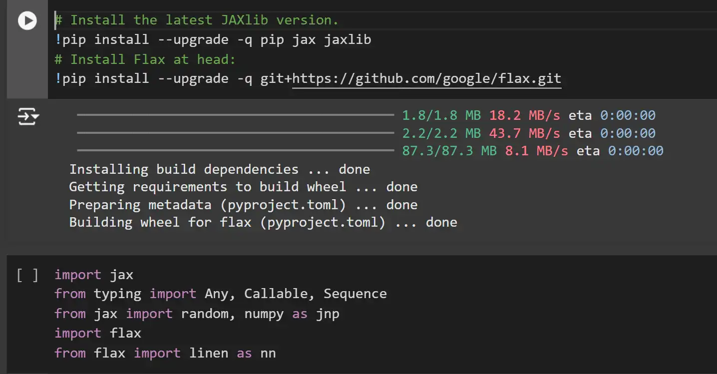
Before building models with Flax, it’s essential to set up your development environment with the necessary libraries. We’ll install the latest versions of JAX, JAXlib, and Flax. JAX is the backbone that provides high-performance numerical computing, while Flax builds upon it to offer a flexible neural network framework.

# Install the latest JAXlib version.
!pip install --upgrade -q pip jax jaxlib
# Install Flax at head:
!pip install --upgrade -q git+https://github.com/google/flax.git


import jax
from typing import Any, Callable, Sequence
from jax import random, numpy as jnp
import flax
from flax import linen as nn

Explanation:

• JAX and JAXlib: JAX is a library for high-performance numerical computing and automatic differentiation, while JAXlib provides the low-level implementations required by JAX.
• Flax: A neural network library built on top of JAX, offering a flexible and efficient API for building models.
• Flax’s Linen API: Imported as nn, Linen is Flax’s high-level API for defining neural network layers and models.

Flax Fundamentals: Linear Regression Example

Linear regression is a foundational machine learning technique used to model the relationship between a dependent variable and one or more independent variables. In Flax, we can implement linear regression using a single dense (fully connected) layer.

Model Instantiation

First, let’s instantiate a dense layer with Flax’s Linen API.

# We create one dense layer instance (taking 'features' parameter as input)
model = nn.Dense(features=5)

Explanation:

• nn.Dense: Represents a dense (fully connected) neural network layer with a specified number of output features. Here, we’re creating a dense layer with 5 output features.

Parameter Initialization

In Flax, model parameters are not stored within the model itself. Instead, you need to initialize them using a random key and dummy input data. This process leverages Flax’s lazy initialization, where parameter shapes are inferred based on the input data.

key1, key2 = random.split(random.key(0))
x = random.normal(key1, (10,)) # Dummy input data
params = model.init(key2, x) # Initialization call
jax.tree_util.tree_map(lambda x: x.shape, params) # Checking output shapes

Explanation:

• Random Key Splitting: JAX uses pure functions and handles randomness via explicit PRNG keys. We split the initial key into two for independent random number generation.
• Dummy Input Data: A dummy input x with shape (10,) is used to trigger shape inference during parameter initialization.
• model.init: Initializes the model’s parameters based on the input data shape and the random key.
• tree_map: Applies a function to each leaf in the parameter tree to inspect shapes.

Note: JAX and Flax, like NumPy, are row-based systems, meaning that vectors are represented as row vectors and not column vectors. This can be seen in the shape of the kernel here.

Forward Pass

After initializing the parameters, you can perform a forward pass to compute the model’s output for a given input.

model.apply(params, x)

Explanation:

• model.apply: Executes the model’s forward pass using the provided parameters and input data.

Gradient Descent Training

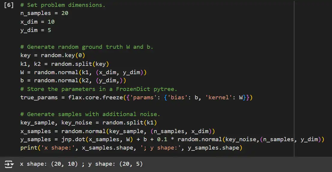
With the model initialized, we can perform gradient descent to train our linear regression model. We’ll generate synthetic data and define a mean squared error (MSE) loss function.

# Set problem dimensions.
n_samples = 20
x_dim = 10
y_dim = 5

# Generate random ground truth W and b.
key = random.key(0)
k1, k2 = random.split(key)
W = random.normal(k1, (x_dim, y_dim))
b = random.normal(k2, (y_dim,))
# Store the parameters in a FrozenDict pytree.
true_params = flax.core.freeze({'params': {'bias': b, 'kernel': W}})

# Generate samples with additional noise.
key_sample, key_noise = random.split(k1)
x_samples = random.normal(key_sample, (n_samples, x_dim))
y_samples = jnp.dot(x_samples, W) + b + 0.1 * random.normal(key_noise, (n_samples, y_dim))
print('x shape:', x_samples.shape, '; y shape:', y_samples.shape)

Explanation:

• Problem Dimensions: Defines the number of samples (n_samples), input dimension (x_dim), and output dimension (y_dim).
• Ground Truth Parameters: Randomly initializes the true weights W and biases b used to generate synthetic target data.
• FrozenDict: Flax uses FrozenDict to ensure immutability of parameters.
• Data Generation: Creates synthetic input data x_samples and target data y_samples with added noise to simulate real-world scenarios.

Defining the MSE Loss Function

Next, we’ll define the mean squared error (MSE) loss function and perform gradient descent using JAX’s JIT compilation for efficiency.

# Define the MSE loss function.
@jax.jit
def mse(params, x_batched, y_batched):
    # Define the squared loss for a single pair (x, y)
    def squared_error(x, y):
        pred = model.apply(params, x)
        return jnp.inner(y - pred, y - pred) / 2.0
    # Vectorize the previous to compute the average of the loss on all samples.
    return jnp.mean(jax.vmap(squared_error)(x_batched, y_batched), axis=0)

Explanation:

• @jax.jit: JIT-compiles the mse function for optimized performance.
• squared_error: Computes the squared error between predictions and true values.
• jax.vmap: Vectorizes the squared_error function to apply it across all samples efficiently.
• Mean Squared Error: Calculates the average loss over all samples.

Gradient Descent Parameters and Update Function

We’ll set the learning rate and define functions to compute gradients and update model parameters.

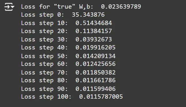
learning_rate = 0.3  # Gradient step size.
print('Loss for "true" W,b: ', mse(true_params, x_samples, y_samples))
loss_grad_fn = jax.value_and_grad(mse)

@jax.jit
def update_params(params, learning_rate, grads):
  params = jax.tree_util.tree_map(
      lambda p, g: p - learning_rate * g, params, grads)
  return params

for i in range(101):
  # Perform one gradient update.
  loss_val, grads = loss_grad_fn(params, x_samples, y_samples)
  params = update_params(params, learning_rate, grads)
  if i % 10 == 0:
    print(f'Loss step {i}: ', loss_val)

Explanation:

• Learning Rate: Determines the step size during parameter updates.
• loss_grad_fn: Uses jax.value_and_grad to compute both the loss value and its gradients with respect to the parameters.
• update_params: Updates the model parameters by subtracting the product of the learning rate and gradients.

Training Loop

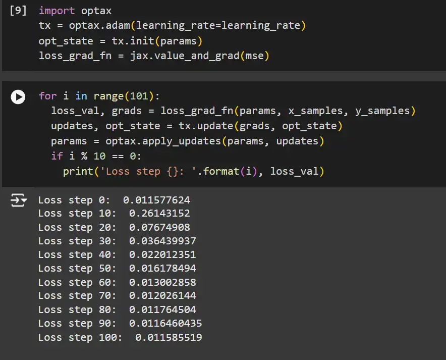
Finally, we’ll execute the training loop, performing parameter updates and monitoring the loss.

import optax
tx = optax.adam(learning_rate=learning_rate)
opt_state = tx.init(params)
loss_grad_fn = jax.value_and_grad(mse)

for i in range(101):
  loss_val, grads = loss_grad_fn(params, x_samples, y_samples)
  updates, opt_state = tx.update(grads, opt_state)
  params = optax.apply_updates(params, updates)
  if i % 10 == 0:
    print('Loss step {}: '.format(i), loss_val)

Explanation:

• Optax Optimizer: Initializes the Adam optimizer with the specified learning rate.
• Optimizer State: Maintains the state required by the optimizer (e.g., momentum terms for Adam).
• tx.update: Computes parameter updates based on gradients and the optimizer state.
• optax.apply_updates: Applies the computed updates to the model parameters.
• Training Loop: Iterates through training steps, updating parameters and monitoring loss.

Benefits of Using Optax:

• Simplicity: Abstracts away manual gradient updates, reducing boilerplate code.
• Flexibility: Supports a wide range of optimization algorithms and gradient transformations.
• Composability: Allows composing simple gradient transformations into more complex optimizers.

Serialization: Saving and Loading Models

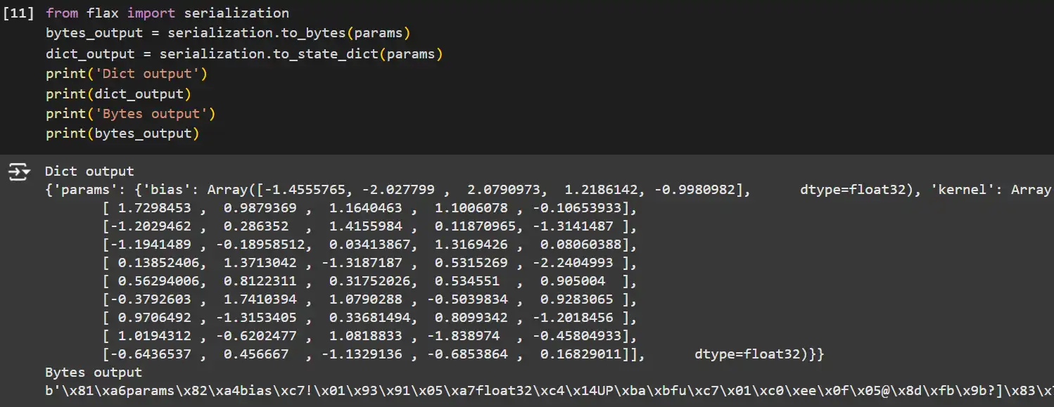
After training, you may want to save your model’s parameters for later use or deployment. Flax provides robust serialization utilities to facilitate this process.

from flax import serialization

# Serialize parameters to bytes.
bytes_output = serialization.to_bytes(params)
# Serialize parameters to a dictionary.
dict_output = serialization.to_state_dict(params)

print('Dict output')
print(dict_output)
print('Bytes output')
print(bytes_output)

Explanation:

• serialization.to_bytes: Converts the parameter tree to a byte string, suitable for storage or transmission.
• serialization.to_state_dict: Converts the parameter tree to a dictionary, making it easy to save as JSON or other human-readable formats.

Deserializing the Model

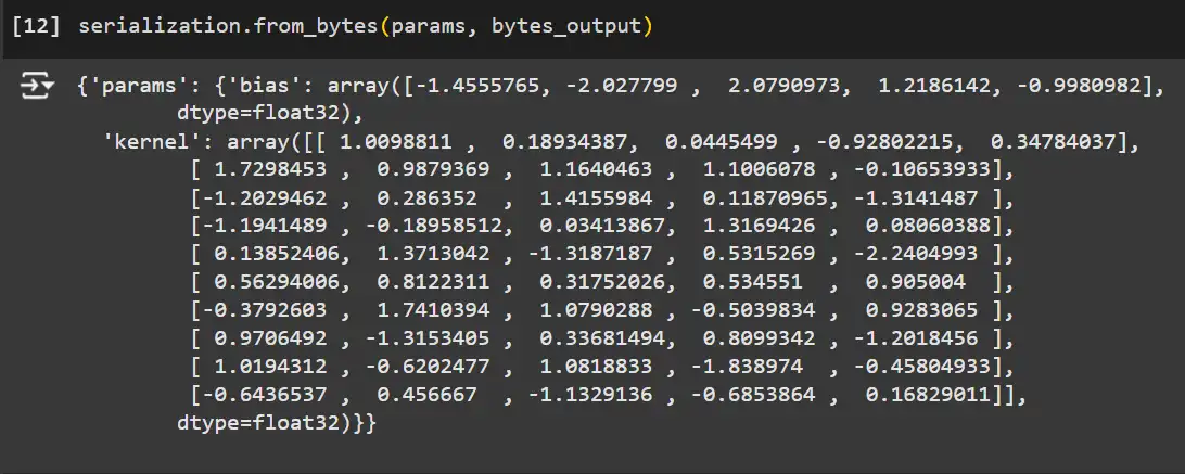
Using the from_bytes method with a parameter template to load the model parameters back.

# Load the model back using the serialized bytes.
loaded_params = serialization.from_bytes(params, bytes_output)

Defining Custom Models

Flax’s flexibility shines when defining custom models beyond simple linear regressions. This section’ll explore how to create custom multi-layer perceptrons (MLPs) and manage state within your models.

Module Basics

Modules in Flax are subclasses of nn.Module and represent layers or entire models. Here’s how to define a custom MLP with a sequence of dense layers and activation functions.

class ExplicitMLP(nn.Module):
  features: Sequence(int)

  def setup(self):
    # we automatically know what to do with lists, dicts of submodules
    self.layers = (nn.Dense(feat) for feat in self.features)
    # for single submodules, we would just write:
    # self.layer1 = nn.Dense(feat1)

  def __call__(self, inputs):
    x = inputs
    for i, lyr in enumerate(self.layers):
      x = lyr(x)
      if i != len(self.layers) - 1:
        x = nn.relu(x)
    return x

key1, key2 = random.split(random.key(0), 2)
x = random.uniform(key1, (4,4))

model = ExplicitMLP(features=(3,4,5))
params = model.init(key2, x)
y = model.apply(params, x)

print('initialized parameter shapes:\n', jax.tree_util.tree_map(jnp.shape, flax.core.unfreeze(params)))
print('output:\n', y)

Explanation:

• ExplicitMLP: A simple multi-layer perceptron with specified features for each layer.
• setup(): Register’s submodules (dense layers) that Flax tracks for parameter initialization and serialization.
• __call__(): Defines the forward pass, applying each layer and a ReLU activation except for the last layer.

Attempting to call the model directly without using apply will result in an error:

try:
    y = model(x)  # Returns an error
except AttributeError as e:
    print(e)

Explanation:

• model.apply: Flax’s functional API requires applying to execute the model’s forward pass with given parameters.

Using the @nn.compact Decorator

An alternative and more concise way to define submodules is by using the @nn.compact decorator within the __call__ method.

class SimpleMLP(nn.Module):
  features: Sequence(int)

  @nn.compact
  def __call__(self, inputs):
    x = inputs
    for i, feat in enumerate(self.features):
      x = nn.Dense(feat, name=f'layers_{i}')(x)
      if i != len(self.features) - 1:
        x = nn.relu(x)
      # providing a name is optional though!
      # the default autonames would be "Dense_0", "Dense_1", ...
    return x

key1, key2 = random.split(random.key(0), 2)
x = random.uniform(key1, (4,4))

model = SimpleMLP(features=(3,4,5))
params = model.init(key2, x)
y = model.apply(params, x)

print('initialized parameter shapes:\n', jax.tree_util.tree_map(jnp.shape, flax.core.unfreeze(params)))
print('output:\n', y)

Explanation:

• @nn.compact: A decorator that allows defining submodules and parameters within the __call__ method, enabling a more concise and readable model definition.
• Naming Submodules: Optionally provides names to submodules for clarity; otherwise, Flax auto-generates names like “Dense_0”, “Dense_1”, etc.

Differences Between setup and @nn.compact:

• setup Method:
  • Allows defining submodules outside the __call__ method.
  • Useful for modules with multiple methods or dynamic structures.
• @nn.compact Decorator:
  • Enables defining submodules within the __call__ method.
  • More concise for simple and fixed architectures.

Module Parameters

Sometimes, you might need to define custom layers not provided by Flax. Here’s how to create a simple dense layer from scratch using the @nn.compact approach.

class SimpleDense(nn.Module):
    features: int
    kernel_init: Callable = nn.initializers.lecun_normal()
    bias_init: Callable = nn.initializers.zeros_init()

    @nn.compact
    def __call__(self, inputs):
        kernel = self.param('kernel',
                            self.kernel_init,  # Initialization function
                            (inputs.shape(-1), self.features))  # Shape info.
        y = jnp.dot(inputs, kernel)
        bias = self.param('bias', self.bias_init, (self.features,))
        y = y + bias
        return y

key1, key2 = random.split(random.key(0), 2)
x = random.uniform(key1, (4, 4))

model = SimpleDense(features=3)
params = model.init(key2, x)
y = model.apply(params, x)

print('initialized parameters:\n', params)
print('output:\n', y)

Explanation:

• Custom Parameters: Uses self.param to register custom parameters (kernel and bias).
• Initialization Functions: Specifies how each parameter is initialized.
• Manual Computation: Performs the dense computation manually using jnp.dot.

Key Points:

• self.param: Registers a parameter with a name, initialization function, and shape.
• Manual Parameter Management: Provides granular control over parameter definitions and initializations.

Variables and Collections of Variables

In addition to parameters, neural networks often maintain state variables, such as running statistics in batch normalization. Flax allows you to manage these variables using the variable method.

Example: Bias Adder with Running Mean

class BiasAdderWithRunningMean(nn.Module):
    decay: float = 0.99

    @nn.compact
    def __call__(self, x):
        # Check if 'mean' variable is initialized.
        is_initialized = self.has_variable('batch_stats', 'mean')
        # Initialize running average of the mean.
        ra_mean = self.variable('batch_stats', 'mean',
                                lambda s: jnp.zeros(s),
                                x.shape(1:))
        # Initialize bias parameter.
        bias = self.param('bias', lambda rng, shape: jnp.zeros(shape), x.shape(1:))
        if is_initialized:
            ra_mean.value = self.decay * ra_mean.value + (1.0 - self.decay) * jnp.mean(x, axis=0, keepdims=True)

        return x - ra_mean.value + bias

# Initialize and apply the model.
key1, key2 = random.split(random.key(0), 2)
x = jnp.ones((10, 5))
model = BiasAdderWithRunningMean()
variables = model.init(key1, x)
print('initialized variables:\n', variables)
y, updated_state = model.apply(variables, x, mutable=('batch_stats'))
print('updated state:\n', updated_state)

Explanation:

• self.variable: Registers a mutable variable (mean) under the ‘batch_stats’ collection.
• State Initialization: Initializes running mean with zeros.
• State Update: Updates the running mean during the forward pass if already initialized.
• Mutable State: Specifies which collections are mutable during the forward pass using the mutable argument in apply.

Managing Optimizer and Model State

Handling both parameters and state variables (like running means) can be complex. Here’s an example of integrating parameter updates with state variable updates using Optax.

for val in (1.0, 2.0, 3.0):
  x = val * jnp.ones((10,5))
  y, updated_state = model.apply(variables, x, mutable=('batch_stats'))
  old_state, params = flax.core.pop(variables, 'params')
  variables = flax.core.freeze({'params': params, **updated_state})
  print('updated state:\n', updated_state) # Shows only the mutable part

from functools import partial

@partial(jax.jit, static_argnums=(0, 1))
def update_step(tx, apply_fn, x, opt_state, params, state):

  def loss(params):
    y, updated_state = apply_fn({'params': params, **state},
                                x, mutable=list(state.keys()))
    l = ((x - y) ** 2).sum()
    return l, updated_state

  (l, state), grads = jax.value_and_grad(loss, has_aux=True)(params)
  updates, opt_state = tx.update(grads, opt_state)
  params = optax.apply_updates(params, updates)
  return opt_state, params, state

x = jnp.ones((10,5))
variables = model.init(random.key(0), x)
state, params = flax.core.pop(variables, 'params')
del variables
tx = optax.sgd(learning_rate=0.02)
opt_state = tx.init(params)

for _ in range(3):
  opt_state, params, state = update_step(tx, model.apply, x, opt_state, params, state)
  print('Updated state: ', state)

Explanation:

• update_step Function: A JIT-compiled function that updates both parameters and state variables.
• Loss Function: Computes the loss and updates state variables simultaneously.
• Gradient Computation: Uses jax.value_and_grad to compute gradients with respect to parameters.
• Optax Updates: Applies optimizer updates to the parameters.
• Training Loop: Iterates through training steps, updating parameters and state variables.

Note: The function signature can be verbose and may not work with jax.jit() directly because some function arguments are not “valid JAX types.” Flax provides a convenient wrapper called TrainState to simplify this process. Refer to flax.training.train_state.TrainState for more information.

Exporting to TensorFlow’s SavedModel with jax2tf

JAX released an experimental converter called jax2tf, which allows converting trained Flax models into TensorFlow SavedModel format (so it can be used for TF Hub, TF.lite, TF.js, or other downstream applications). The repository contains more documentation and has various examples for Flax.

Conclusion

Flax is a versatile and powerful neural network library that leverages JAX’s high-performance capabilities. From setting up simple linear regression models to defining complex custom architectures and managing state, Flax provides a flexible framework for research and production environments.

In this guide, we covered:

• Environment Setup: Installing JAX, JAXlib, and Flax.
• Linear Regression: Implementing and training a simple linear model.
• Optimization with Optax: Streamlining the training process using advanced optimizers.
• Serialization: Saving and loading model parameters efficiently.
• Custom Models: Building custom neural network architectures with state management.

By mastering these fundamentals, you’re well-equipped to harness Flax’s full potential in your machine-learning projects. Whether you’re conducting academic research, developing production-ready models, or exploring innovative architectures, Flax offers the tools and flexibility to support your endeavours.

Also, if you are looking for an ai/ML course online, then explore: Certified ai & ML BlackBelt PlusProgram

Key Takeaways

1. Flax is a flexible, high-performance neural network library built on JAX, offering modularity and composability for deep learning models.
2. It follows a functional programming paradigm, enhancing models’ reproducibility, debugging, and maintainability.
3. Flax integrates seamlessly with JAX, utilizing its optimization and parallelization capabilities for high-speed computation.
4. The Linen API and `@nn.compact` decorator simplify defining and managing neural network layers and parameters.
5. Flax provides utilities for state management, model serialization, and efficient training using composable optimizers like Optax.

The media shown in this article is not owned by Analytics Vidhya and is used at the Author’s discretion.

Frequently Asked Questions