
Image by Author
Sparse data refers to datasets with many features with zero values. It can cause problems in different fields, especially in machine learning.
Sparse data can occur as a result of inappropriate feature engineering methods. For instance, using a one-hot encoding that creates a large number of dummy variables.
Sparsity can be calculated by taking the ratio of zeros in a dataset to the total number of elements. Addressing sparsity will affect the accuracy of your machine-learning model.
Also, we should distinguish sparsity from missing data. Missing data simply means that some values are not available. In sparse data, all values are present, but most are zero.
Also, sparsity causes unique challenges for machine learning. To be exact, it causes overfitting, losing good data, memory problems, and time problems.
This article will explore these common problems related to sparse data. Then we will cover the techniques used to handle this issue.
Finally, we will apply different machine learning models to the sparse data and explain why these models are suitable for sparse data.
Throughout the article, I will predominantly use the scikit-learn library, and if you wish to modify the code and arguments, I will provide the official documentation links too.
Now let’s start with the common problems with sparse data.
Sparse data can pose unique challenges for data analysis. We already mentioned that some of the most common issues include overfitting, losing good data, memory problems, and time problems.
Now, let’s have a detailed look at each.
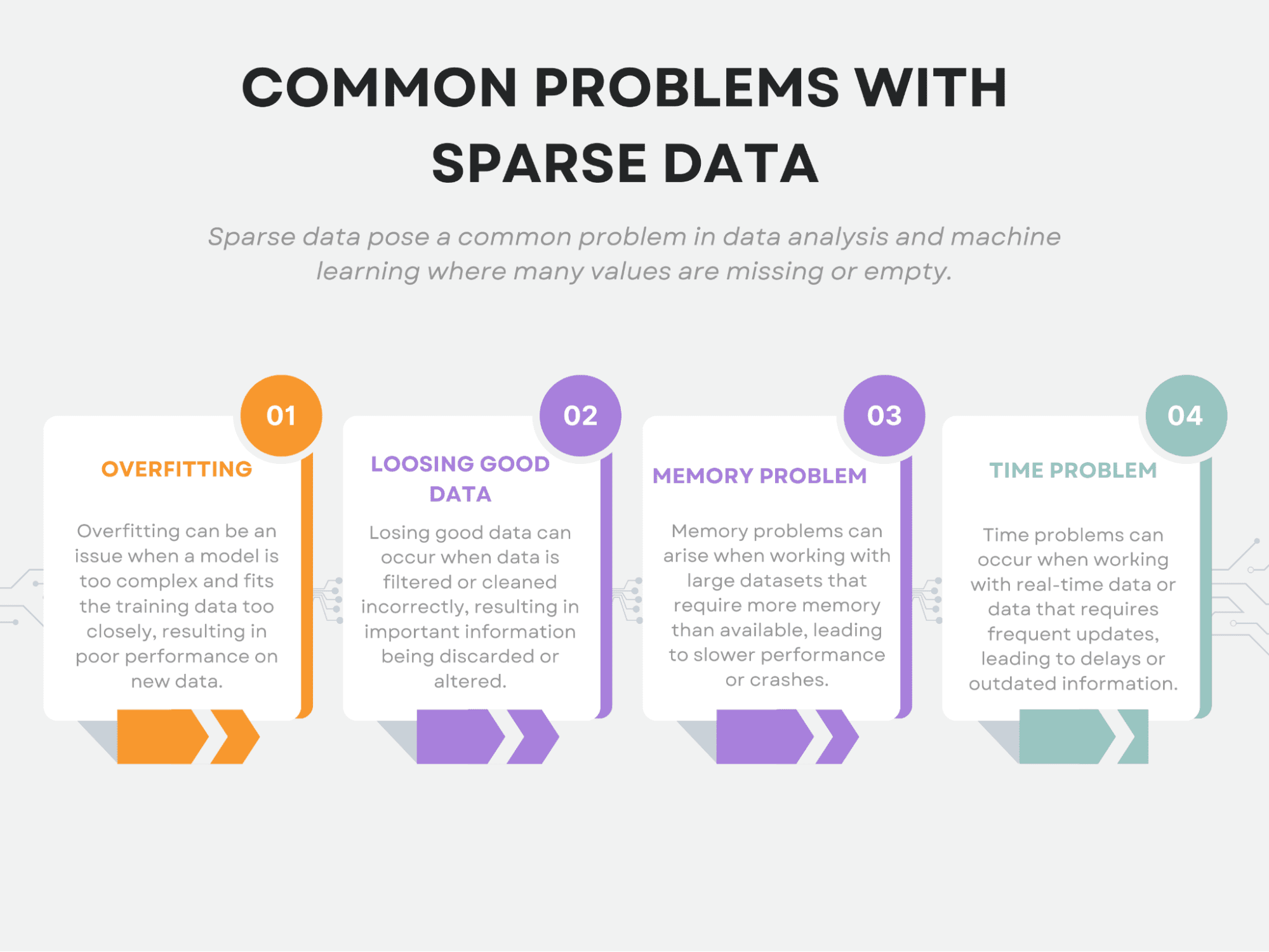

Image by Author
Overfitting
Overfitting occurs when a model becomes too complex and starts to capture noise in the data instead of the underlying patterns.
In sparse data, there may be a large number of features, but only a few of them are actually relevant to the analysis. This can make it difficult to identify which features are important and which ones are not.
As a result, a model may overfit to noise in the data and perform poorly on new data.
If you are new to machine learning or want to know more, you can do that in the scikit-learn documentation about overfitting.
Losing Good Data
One of the biggest problems with sparse data is that it can lead to the loss of potentially useful information.
When we have very limited data, it becomes more difficult to identify meaningful patterns or relationships in that data. This is because the noise and randomness inherent to any data set can more easily obscure essential features when the data is sparse.
Furthermore, because the amount of data available is limited, there is a higher chance that we will miss out on some of the truly valuable patterns or relationships in the data. This is especially true in cases where the data is sparse due to a lack of sampling, as opposed to simply being missing. In such cases, we may not even be aware of the missing data points and thus may not realize we are losing valuable information.
That’s why if too many features are removed, or the data is compressed too much, important information may be lost, resulting in a less accurate model.
Memory Problem
Memory problems can arise due to the large size of the dataset. Sparse data often results in many features, and storing this data can be computationally expensive. This can limit the amount of data that can be processed at once or require significant computing resources.
Here you can see different strategies to scale your data by using scikit-learn.
Time Problem
The time problem can also occur due to the large size of the dataset. Sparse data may require longer processing times, especially when dealing with a large number of features. This can limit the speed at which data can be processed, which can be problematic in time-sensitive applications.
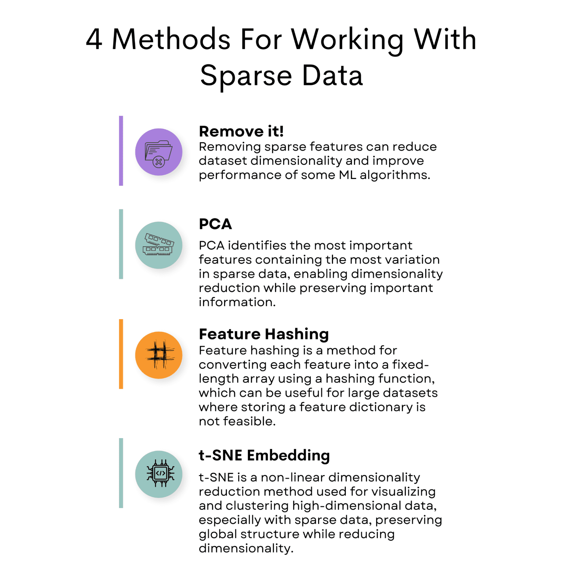

Image by Author
Sparse data poses a challenge in data analysis due to its low occurrence of non-zero values. However, there are several methods available to mitigate this issue.
One common approach is removing the feature causing sparsity in the dataset.
Another option is to use Principal Component Analysis (PCA) to reduce the dimensionality of the dataset while retaining important information.
Feature hashing is another technique that can be employed, which involves mapping features to a fixed-length vector.
T-Distributed Stochastic Neighbor Embedding (t-SNE) is another useful method that can be utilized to visualize high-dimensional datasets.
In addition to these techniques, selecting a suitable machine learning model that can handle sparse data, such as SVM or logistic regression, is crucial.
By implementing these strategies, one can effectively address the challenges associated with sparse data in data analysis.
Now let’s start with the tactics used to reduce sparse data first, then we will go deeper into the models.
Remove it!
When working with sparse data, one approach is to remove features that contain mostly zero values. This can be done by setting a threshold on the percentage of non-zero values in each feature. Any feature that falls below this threshold can be removed from the dataset.
This approach can help reduce the dimensionality of the dataset and improve the performance of certain machine learning algorithms.
Code Example
In this example, we set the dimensions of the dataset, as well as the sparsity level, which determines how many values in the dataset will be zero.
Then, we generate random data with the specified sparsity level to check whether our method works or not. At this step, we calculate the sparsity to compare afterward.
Next, the code sets the number of zeros to remove and randomly removes a specific number of zeros from the dataset. Then we recalculate the sparsity of the modified dataset to check whether our method works or not.
Finally, we recalculate the sparsity to see the changes.
Here is the code.
import numpy as np

# Set the dimensions of the dataset
num_rows = 1000
num_cols = 100

# Set the sparsity level of the dataset
sparsity = 0.9

# Generate random data with the specified sparsity level
data = np.random.random((num_rows, num_cols))
data[data < sparsity] = 0

# Calculate the sparsity of the dataset
num_zeros = (data == 0).sum()
total_elements = data.shape[0] * data.shape[1]
sparsity = num_zeros / total_elements

print(f"The sparsity of the dataset before removal {sparsity:.4f}")

# Set the number of zeros to remove
num_zeros_to_remove = 50000

# Remove a specific number of zeros randomly from the dataset
zero_indices = np.argwhere(data == 0)
zeros_to_remove = np.random.choice(
    zero_indices.shape[0], num_zeros_to_remove, replace=False
)
data[
    zero_indices[zeros_to_remove, 0], zero_indices[zeros_to_remove, 1]
] = np.nan

# Calculate the sparsity of the modified dataset

num_zeros = (data == 0).sum()
total_elements = data.shape[0] * data.shape[1]
sparsity = num_zeros / total_elements

print(
    "Sparsity after removing {} zeros:".format(num_zeros_to_remove), sparsity
)
Here is the output.


PCA
PCA is a popular technique for dimensionality reduction. It identifies the principal components of the data, which are the directions in which the data varies the most.
These principal components can then be used to represent the data in a lower-dimensional space.
In the context of sparse data, PCA can be used to identify the most important features that contain the most variation in the data.
By selecting only these features, we can reduce the dimensionality of the dataset while still retaining most of the important information.
You can implement PCA by using the sci-kit learn library, as we will do it next in the code example. Here is the official documentation if you want to learn more about it.
Code Example
To apply PCA to sparse data, we can use the scikit-learn library in Python.
The library provides a PCA class that we can use to fit a PCA model to the data and transform it into lower-dimensional space.
In the first section of the following code, we create a dataset as we did in the previous section, with a given dimension and sparsity.
In the second section, we will apply PCA to reduce the dimension of the dataset to 10. After that, we will recalculate the sparsity.
Here is the code.
import numpy as np

# Set the dimensions of the dataset
num_rows = 1000
num_cols = 100

# Set the sparsity level of the dataset
sparsity = 0.9

# Generate random data with the specified sparsity level
data = np.random.random((num_rows, num_cols))
data[data < sparsity] = 0

# Calculate the sparsity of the dataset
num_zeros = (data == 0).sum()
total_elements = data.shape[0] * data.shape[1]
sparsity = num_zeros / total_elements

print(f"The sparsity of the dataset before removal {sparsity:.4f}")

# Apply PCA to the dataset
pca = PCA(n_components=10)
data_pca = pca.fit_transform(data)
# Calculate the sparsity of the reduced dataset
num_zeros = (data_pca == 0).sum()
total_elements = data_pca.shape[0] * data_pca.shape[1]
sparsity = num_zeros / total_elements

print(f"Sparsity after PCA: {sparsity:.4f}")
Here is the output.


Feature Hashing
Another method for working with sparse data is called feature hashing. This approach converts each feature into a fixed-length array of values using a hashing function.
The hashing function maps each input feature to a set of indices in the fixed-length array. The values are summed together if multiple input features are mapped to the same index. Feature hashing can be useful for large datasets where storing a large feature dictionary may not be feasible.
We will cover this together in the next section, yet if you want to dig deeper into it, here you can see the official documentation of the feature hasher in the scikit-learn library.
Code Example
Here, we again use the same method in dataset creation.
Then we apply feature hashing to the dataset using the FeatureHasher class from scikit-learn.
We specify the number of output features with the n_features parameter and the input type as a dictionary with the input_type parameter.
We then transform the input data into hashed arrays using the transform method of the FeatureHasher object.
Finally, we calculate the sparsity of the resulting dataset.
Here is the code.
import numpy as np

# Set the dimensions of the dataset
num_rows = 1000
num_cols = 100

# Set the sparsity level of the dataset
sparsity = 0.9

# Generate random data with the specified sparsity level
data = np.random.random((num_rows, num_cols))
data[data < sparsity] = 0

# Calculate the sparsity of the dataset
num_zeros = (data == 0).sum()
total_elements = data.shape[0] * data.shape[1]
sparsity = num_zeros / total_elements

print(f"The sparsity of the dataset before removal {sparsity:.4f}")

# Apply feature hashing to the dataset
hasher = FeatureHasher(n_features=10, input_type="dict")
data_dict = [
    dict(("feature" + str(i), val) for i, val in enumerate(row))
    for row in data
]
data_hashed = hasher.transform(data_dict).toarray()

# Calculate the sparsity of the reduced dataset
num_zeros = (data_hashed == 0).sum()
total_elements = data_hashed.shape[0] * data_hashed.shape[1]
sparsity = num_zeros / total_elements

print(f"Sparsity after feature hashing: {sparsity:.4f}")
Here is the output.


t-SNE Embedding
t-SNE (t-Distributed Stochastic Neighbor Embedding) is a non-linear dimensionality reduction technique used to visualize high-dimensional data. It reduces the dimensionality of the data while preserving its global structure and has become a popular tool in machine learning for visualizing and clustering high-dimensional data.
t-SNE is particularly useful for working with sparse data because it can effectively reduce the dimensionality of the data while maintaining its structure. The t-SNE algorithm works by calculating pairwise distances between data points in high- and low-dimensional spaces. It then minimizes the difference between these distances in high- and low-dimensional space.
To use t-SNE with sparse data, the data must first be converted into a dense matrix. This can be done using various techniques, such as PCA or feature hashing. Once the data has been converted, t-SNE can be high-x to obtain a low-dimensional embedding of the data.
Also, if you are curious about t-SNE, here is the official documentation of the scikit-learn to see more.
Code Example
The following code first sets the dimensions of the dataset and the sparsity level, generates random data with the specified sparsity level, and calculates the sparsity of the dataset before t-SNE is applied, as we did in the previous examples.
It then applies t-SNE to the dataset with 3 components and calculates the sparsity of the resulting t-SNE embedding. Finally, it prints out the sparsity of the t-SNE embedding.
Here is the code.
import numpy as np

# Set the dimensions of the dataset
num_rows = 1000
num_cols = 100

# Set the sparsity level of the dataset
sparsity = 0.9

# Generate random data with the specified sparsity level
data = np.random.random((num_rows, num_cols))
data[data < sparsity] = 0

# Calculate the sparsity of the dataset
num_zeros = (data == 0).sum()
total_elements = data.shape[0] * data.shape[1]
sparsity = num_zeros / total_elements

print(f"The sparsity of the dataset before removal {sparsity:.4f}")

# Apply t-SNE to the dataset
tsne = TSNE(n_components=3)
data_tsne = tsne.fit_transform(data)

# Calculate the sparsity of the t-SNE embedding
num_zeros = (data_tsne == 0).sum()
total_elements = data_tsne.shape[0] * data_tsne.shape[1]
sparsity = num_zeros / total_elements

print(f"Sparsity after t-SNE: {sparsity:.4f}")
Here is the output.


Now that we have addressed the challenges of working with sparse data, we can explore machine learning models specifically designed to perform well with sparse data.
These models can handle the unique characteristics of sparse data, such as a high number of features with many zeros and limited information, which can make it challenging to achieve accurate predictions with traditional models.
By using models designed explicitly for sparse data, we can ensure that our predictions are more precise and reliable.
Now let’s talk about the models good for sparse data.
SVC (Support Vector Classifier)
SVC (Support Vector Classifier) with the linear kernel can perform well with sparse data because it uses a subset of training points, known as support vectors, to make predictions. This means it can handle high-dimensional, sparse data efficiently.
You can use Support Vector for regression, too.
I explained the Support Vector Machine here if you want to learn more about the Support Vector algorithm, both classification and regression.
Logistic Regression
This can also work well with sparse data because logistic regression uses a regularization term to control the model complexity, which can help prevent overfitting on sparse datasets.
If you want to learn more about logistic regression and also for other classification algorithms, here is the Overview of Machine Learning Algorithms: Classification.
KNeighboursClassifier
This algorithm can work well with sparse data since it computes distances between data points and can handle high-dimensional data.
You can see KNN and other machine learning algorithms here that you should know for data science.
MLPClassifier
The MLPClassifier can perform well with sparse data when the input data is standardized, as it uses gradient descent for optimization.
Here you can see the implementation of MLP Classifier, along witha bunch of other algorithms, with the help of ChatGPT.
DecisionTreeClassifier
It can work well with sparse data when the number of features is small. If you do not know about decision trees, I explained decision trees and random forests here, which will be our final model for analyzing the models for sparse data.
RandomForestClassifier
The RandomForestClassifier can work well with sparse data when the number of features is small.
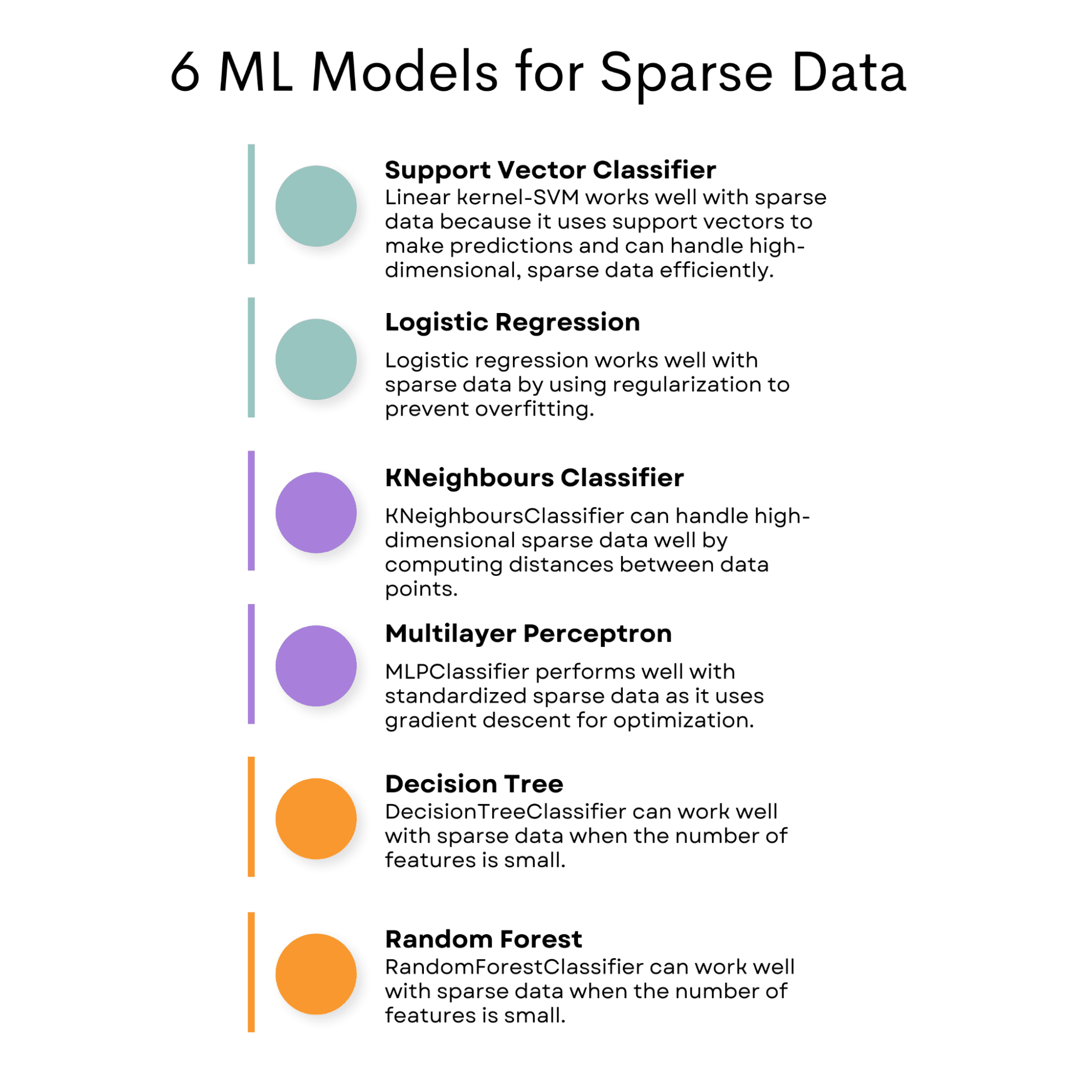

Image by Author
Now, I will show you how these models perform on the generated data. But, I will add another algorithm to see whether these algorithms will outperform this algorithm (which is typically not good for sparse data) or not.
Code Example
In this section, we will test multiple machine learning models on a sparse dataset, which is a dataset with a lot of empty or zero values.
We will calculate the sparsity of the dataset and evaluate the models using the F1 score.
Then, we will create a data frame with the F1 scores for each model to compare their performance. Also, we will filter out any warnings that may appear during the evaluation process.
import numpy as np
from scipy.sparse import random
import numpy as np
from scipy.sparse import random
from sklearn.model_selection import train_test_split
from sklearn.metrics import f1_score
from sklearn.svm import SVC
from sklearn.linear_model import LogisticRegression, Lasso
from sklearn.cluster import KMeans
from sklearn.neighbors import KNeighborsClassifier
from sklearn.neural_network import MLPClassifier
from sklearn.datasets import make_classification
from sklearn.preprocessing import StandardScaler
from sklearn.model_selection import train_test_split
from sklearn.exceptions import ConvergenceWarning
import warnings

# Generate a sparse dataset
X = random(1000, 20, density=0.1, format="csr", random_state=42)
y = np.random.randint(2, size=1000)

# Calculate the sparsity of the dataset
sparsity = 1.0 - X.nnz / float(X.shape[0] * X.shape[1])
print("Sparsity:", sparsity)

X_train, X_test, y_train, y_test = train_test_split(
    X, y, test_size=0.2, random_state=42
)

# Train and evaluate multiple classifiers
classifiers = [
    SVC(kernel="linear"),
    LogisticRegression(),
    KMeans(
        n_clusters=2,
        init="k-means++",
        max_iter=100,
        random_state=42,
        algorithm="full",
    ),
    KNeighborsClassifier(n_neighbors=5),
    MLPClassifier(
        hidden_layer_sizes=(100, 50),
        max_iter=1000,
        alpha=0.01,
        solver="sgd",
        verbose=0,
        random_state=21,
        tol=0.000000001,
    ),
    DecisionTreeClassifier(),
    RandomForestClassifier(),
]

# Create an empty DataFrame with column names
df = pd.DataFrame(columns=["Classifier", "F1 Score"])

# Filter out the specific warning
warnings.filterwarnings(
    "ignore", category=ConvergenceWarning
)  # Filter warning that mlp classifier will possibly print out.

for clf in classifiers:
    clf.fit(X_train, y_train)
    y_pred = clf.predict(X_test)
    f1 = f1_score(y_test, y_pred)
    df = pd.concat(
        [
            df,
            pd.DataFrame(
                {"Classifier": [type(clf).__name__], "F1 Score": [f1]}
            ),
        ],
        ignore_index=True,
    )
df = df.sort_values(by="F1 Score", ascending=True)
df
Here is the output.
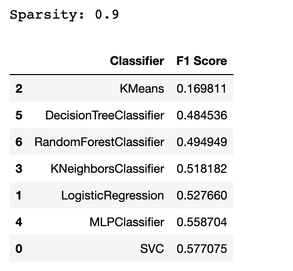

By now, you might catch an algorithm that is not well-suited for the sparse data. Yes, the answer is the KMeans. But why?
KMeans is typically not well suited for sparse data because it is based on distance measures, which can be problematic with high-dimensional, sparse data.
There are also some algorithms that we can’t even try. For instance, if you try to include the GaussianNB classifier in this list, you will get an error. It suggests that the GaussianNB classifier expects dense data instead of sparse data. This is because the GaussianNB classifier assumes that the input data follows Gaussian distribution and is unsuitable for sparse data.
In conclusion, working with sparse data can be challenging due to various problems like overfitting, losing good data, memory, and time problems.
However, several methods are available for working with sparse features, including removing features, using PCA, and feature hashing.
Moreover, certain machine learning models like SVM, Logistic Regression, Lasso, Decision Tree, Random Forest, MLP, and k-nearest neighbors are well-suited for handling sparse data.
These models have been designed to handle high-dimensional and sparse data efficiently, making them the best choices for sparse data problems. Using these methods and models can improve your model’s accuracy and save time and resources.
Nate Rosidi is a data scientist and in product strategy. He’s also an adjunct professor teaching analytics, and is the founder of StrataScratch, a platform helping data scientists prepare for their interviews with real interview questions from top companies. Connect with him on Twitter: StrataScratch or LinkedIn.
 NEWSLETTER


