Are you making these mistakes when modeling classification?

Introduction

Evaluating a machine learning model isn’t just the final step, it’s the cornerstone of success. Imagine creating a state-of-the-art model that dazzles with its high accuracy, then finding that it falls apart under real-world pressure. Evaluation is more than ticking off metrics; it’s about ensuring that your model performs consistently in practice. In this article, we’ll discuss common mistakes that can derail even the most promising classification models and reveal best practices that can elevate your model from good to great. Let’s turn your classification modeling tasks into reliable and effective solutions.

Overview

• Building a classification model:Build a robust classification model with step-by-step guidance.
• Identify common mistakes:Identify and avoid common mistakes in classification modeling.
• Understanding Overfitting:Understand overfitting and learn how to avoid it in your models.
• Improve model building skills:Improve your model building skills with best practices and advanced techniques.

Classification Modeling: An Overview

In the classification problem, we try to build a model that predicts the labels of the target variable using independent variables. Since we are working with labeled target data, we will need supervised machine learning algorithms like Logistic Regression, SVM, Decision Tree, etc. We will also look at neural network models to solve the classification problem, identify common mistakes that people can make, and determine how to avoid them.

Building a basic classification model

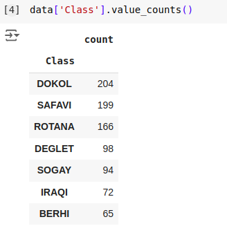
We will demonstrate how to create a fundamental classification model using the Kaggle Dates and Fruits DatasetAbout the dataset: The target variable consists of seven types of dates: Barhee, Deglet Nour, Sukkary, Rotab Mozafati, Ruthana, Safawi, and Sagai. The dataset consists of 898 images of seven different varieties of dates and 34 features were extracted using image processing techniques. The objective is to classify these fruits based on their attributes.

1. Data preparation

import pandas as pd

   from sklearn.model_selection import train_test_split

   from sklearn.preprocessing import StandardScaler

   # Load the dataset

   data = pd.read_excel('/content/Date_Fruit_Datasets.xlsx')

   # Splitting the data into features and target

   x = data.drop('Class', axis=1)

   y = data('Class')

   # Splitting the dataset into training and testing sets

   X_train, X_test, y_train, y_test = train_test_split(x, y, test_size=0.3, random_state=42)

   # Feature scaling

   scaler = StandardScaler()

   X_train = scaler.fit_transform(X_train)

   X_test = scaler.transform(X_test)

2. Logistic regression

from sklearn.linear_model import LogisticRegression

   from sklearn.metrics import accuracy_score

   # Logistic Regression Model

   log_reg = LogisticRegression()

   log_reg.fit(X_train, y_train)

   # Predictions and Evaluation

   y_train_pred = log_reg.predict(X_train)

   y_test_pred = log_reg.predict(X_test)

   # Accuracy

   train_acc = accuracy_score(y_train, y_train_pred)

   test_acc = accuracy_score(y_test, y_test_pred)

   print(f'Logistic Regression - Train Accuracy: {train_acc}, Test Accuracy: {test_acc}')

Results:

- Logistic Regression - Train Accuracy: 0.9538
- Test Accuracy: 0.9222

Read also: Introduction to logistic regression

3. Support Vector Machine (SVM)

from sklearn.svm import SVC

   from sklearn.metrics import accuracy_score

   # SVM

   svm = SVC(kernel="linear", probability=True)

   svm.fit(X_train, y_train)

   # Predictions and Evaluation

   y_train_pred = svm.predict(X_train)

   y_test_pred = svm.predict(X_test)

   train_accuracy = accuracy_score(y_train, y_train_pred)

   test_accuracy = accuracy_score(y_test, y_test_pred)

   print(f"SVM - Train Accuracy: {train_accuracy}, Test Accuracy: {test_accuracy}")

Results:

- SVM - Train Accuracy: 0.9602
- Test Accuracy: 0.9074

Also Read: Guide to Support Vector Machine (SVM) Algorithm

4. Decision tree

from sklearn.tree import DecisionTreeClassifier

   from sklearn.metrics import accuracy_score

   # Decision Tree

   tree = DecisionTreeClassifier(random_state=42)

   tree.fit(X_train, y_train)

   # Predictions and Evaluation

   y_train_pred = tree.predict(X_train)

   y_test_pred = tree.predict(X_test)

   train_accuracy = accuracy_score(y_train, y_train_pred)

   test_accuracy = accuracy_score(y_test, y_test_pred)

   print(f"Decision Tree - Train Accuracy: {train_accuracy}, Test Accuracy: {test_accuracy}")

Results:

- Decision Tree - Train Accuracy: 1.0000
- Test Accuracy: 0.8222

5. Neural networks with TensorFlow

import numpy as np

   from sklearn.preprocessing import LabelEncoder, StandardScaler

   from sklearn.model_selection import train_test_split

   from tensorflow.keras import models, layers

   from tensorflow.keras.callbacks import EarlyStopping, ModelCheckpoint

   # Label encode the target classes

   label_encoder = LabelEncoder()

   y_encoded = label_encoder.fit_transform(y)

   # Train-test split

   X_train, X_test, y_train, y_test = train_test_split(x, y_encoded, test_size=0.2, random_state=42)

   # Feature scaling

   scaler = StandardScaler()

   X_train = scaler.fit_transform(X_train)

   X_test = scaler.transform(X_test)

   # Neural Network

   model = models.Sequential((

     layers.Dense(64, activation='relu', input_shape=(X_train.shape(1),)),

     layers.Dense(32, activation='relu'),

     layers.Dense(len(np.unique(y_encoded)), activation='softmax')  # Ensure output layer size matches number of classes

   ))

   model.compile(optimizer="adam", loss="sparse_categorical_crossentropy", metrics=('accuracy'))

   # Callbacks

   early_stopping = EarlyStopping(monitor="val_loss", patience=10, restore_best_weights=True)

   model_checkpoint = ModelCheckpoint('best_model.keras', monitor="val_loss", save_best_only=True)

   # Train the model

   history = model.fit(X_train, y_train, epochs=100, batch_size=32, validation_data=(X_test, y_test),

                      callbacks=(early_stopping, model_checkpoint), verbose=1)

   # Evaluate the model

   train_loss, train_accuracy = model.evaluate(X_train, y_train, verbose=0)

   test_loss, test_accuracy = model.evaluate(X_test, y_test, verbose=0)

   print(f"Neural Network - Train Accuracy: {train_accuracy}, Test Accuracy: {test_accuracy}")

Results:

- Neural Network - Train Accuracy: 0.9234
- Test Accuracy: 0.9278

Read also: Build your neural network with Tensorflow

Identifying errors

Classification models can face several challenges that can compromise their effectiveness. Recognizing and addressing these issues is essential to building reliable models. Below are some critical aspects to consider:

1. Overfitting and underfitting:
   • Cross-validation: Avoid relying solely on a single training and test split. Use k-fold cross-validation to better evaluate the performance of your model by testing it on multiple data segments.
   • Regularization: Very complex models may overfit by capturing noise in the data. Regularization methods such as pruning or regularization should be used to penalize complexity.
   • Hyperparameter optimization: Exhaustively explore and tune hyperparameters (e.g., via grid or random search) to balance bias and variance.
2. Technical package:
   • Model aggregation: Ensemble methods such as Random Forests or Gradient Boosting combine predictions from multiple models, often resulting in improved generalization. These techniques can capture intricate patterns in the data while mitigating the risk of overfitting by averaging the errors of each model.
3. Class imbalance:
   • Imbalanced classes: In many cases, one class may have less importance than others, leading to biased predictions. Methods such as oversampling, undersampling, or SMOTE should be used depending on the problem.
4. Data leak:
   • Unintentional data leakage: Data leakage occurs when information outside the training set influences the model, leading to inflated performance metrics. It is critical to ensure that the test data remains completely hidden during training and that the features derived from the target variable are carefully managed.

Example of improved logistic regression using grid search

from sklearn.model_selection import GridSearchCV

   # Implementing Grid Search for Logistic Regression

   param_grid = {'C': (0.1, 1, 10, 100), 'solver': ('lbfgs')}

   grid_search = GridSearchCV(LogisticRegression(multi_class="multinomial", max_iter=1000), param_grid, cv=5)

   grid_search.fit(X_train, y_train)

   # Best model

   best_model = grid_search.best_estimator_

   # Evaluate on test set

   test_accuracy = best_model.score(X_test, y_test)

   print(f"Best Logistic Regression - Test Accuracy: {test_accuracy}")

Results:

- Best Logistic Regression - Test Accuracy: 0.9611

Neural Networks with TensorFlow

Let's focus on improving our previous neural network model, focusing on techniques to minimize overfitting and improve generalization.

Early stopping and model checkpoints

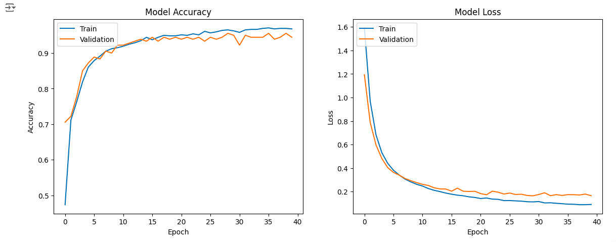
Early stopping stops training when the model validation performance reaches a stable level, preventing overfitting by avoiding excessive learning from noise in the training data.

Model monitoring keeps the best performing model on the validation set throughout training, ensuring that the optimal version of the model is retained even if subsequent training results in overfitting.

import numpy as np

from sklearn.preprocessing import LabelEncoder, StandardScaler

from sklearn.model_selection import train_test_split

from tensorflow.keras import models, layers

from tensorflow.keras.callbacks import EarlyStopping, ModelCheckpoint

# Label encode the target classes

label_encoder = LabelEncoder()

y_encoded = label_encoder.fit_transform(y)

# Train-test split

X_train, X_test, y_train, y_test = train_test_split(x, y_encoded, test_size=0.2, random_state=42)

# Feature scaling

scaler = StandardScaler()

X_train = scaler.fit_transform(X_train)

X_test = scaler.transform(X_test)

# Neural Network

model = models.Sequential((

  layers.Dense(64, activation='relu', input_shape=(X_train.shape(1),)),

  layers.Dense(32, activation='relu'),

  layers.Dense(len(np.unique(y_encoded)), activation='softmax')  # Ensure output layer size matches number of classes

))

model.compile(optimizer="adam", loss="sparse_categorical_crossentropy", metrics=('accuracy'))

# Callbacks

early_stopping = EarlyStopping(monitor="val_loss", patience=10, restore_best_weights=True)

model_checkpoint = ModelCheckpoint('best_model.keras', monitor="val_loss", save_best_only=True)

# Train the model

history = model.fit(X_train, y_train, epochs=100, batch_size=32, validation_data=(X_test, y_test),

                   callbacks=(early_stopping, model_checkpoint), verbose=1)

# Evaluate the model

train_loss, train_accuracy = model.evaluate(X_train, y_train, verbose=0)

test_loss, test_accuracy = model.evaluate(X_test, y_test, verbose=0)

print(f"Neural Network - Train Accuracy: {train_accuracy}, Test Accuracy: {test_accuracy}")

Understanding the importance of different metrics

1. AccuracyWhile important, accuracy may not fully capture a model's performance, particularly when dealing with imbalanced class distributions.
2. LossThe loss function evaluates how well the predicted values ​​align with the actual labels; smaller loss values ​​indicate higher accuracy.
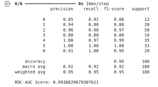
3. Precision, Recall and F1 Score:Precision assesses the accuracy of positive predictions, recall measures the success of the model in identifying all positive cases, and F1 score balances precision and recall.
4. ROC-AUC:The ROC-AUC metric quantifies the model's ability to distinguish between classes regardless of the set threshold.

from sklearn.metrics import classification_report, roc_auc_score

# Predictions

y_test_pred_proba = model.predict(X_test)

y_test_pred = np.argmax(y_test_pred_proba, axis=1)

# Classification report

print(classification_report(y_test, y_test_pred))

# ROC-AUC

roc_auc = roc_auc_score(y_test, y_test_pred_proba, multi_class="ovr")

print(f'ROC-AUC Score: {roc_auc}')

Visualizing model performance

The performance of the model during training can be seen by plotting learning curves for accuracy and loss, which show whether the model is overfitting or underfitting. We use early stopping to avoid overfitting, and this helps generalize to new data.

import matplotlib.pyplot as plt

# Plot training & validation accuracy values

plt.figure(figsize=(14, 5))

plt.subplot(1, 2, 1)

plt.plot(history.history('accuracy'))

plt.plot(history.history('val_accuracy'))

plt.title('Model Accuracy')

plt.xlabel('Epoch')

plt.ylabel('Accuracy')

plt.legend(('Train', 'Validation'), loc="upper left")

# Plot training & validation loss values

plt.subplot(1, 2, 2)

plt.plot(history.history('loss'))

plt.plot(history.history('val_loss'))

plt.title('Model Loss')

plt.xlabel('Epoch')

plt.ylabel('Loss')

plt.legend(('Train', 'Validation'), loc="upper left")

plt.show()

Conclusion

Careful evaluation is crucial to avoid problems such as overfitting and underfitting. Building effective classification models involves more than just choosing and training the right algorithm. Model consistency and reliability can be improved by implementing ensemble methods, regularization, hyperparameter tuning, and cross-validation. While our small dataset may not have experienced significant overfitting, employing these methods ensures that models are robust and accurate, leading to better decision making in practical applications.

Frequently Asked Questions