A Complete Guide to Extrapolation

Introduction

Suppose there is a farmer who observes the progress of crops over several weeks on a daily basis. He observes the growth rates and starts pondering how much more his plants could grow in a few more weeks. From the existing data, he makes a rough forecast of further growth. This operation of assuming the values ​​beyond the range of given data points selected for the purpose is called extrapolation. But it goes without saying that only farmers need to understand extrapolation; anyone who applies data analysis for future-oriented purposes, whether a scientist or an engineer, should do so.

In this article we will delve deeper into the topic of Extrapolation, discussing its need and the methods to carry it out.

Overview

• Understanding the concept of extrapolation.
• Learn about the different methods of extrapolation.
• Recognize the importance and applications of extrapolation in various fields.
• Identify the limitations and challenges associated with extrapolation.
• Learn about best practices for accurate extrapolation.

Extrapolation is a statistical method used to estimate or predict values ​​beyond a given set of known data points. It extends observed trends in data to forecast future outcomes. Unlike interpolation, which predicts values ​​within the range of known data, extrapolation ventures into uncharted territory, often carrying greater risks and uncertainties.

Importance and applications of extrapolation

Extrapolation plays a fundamental role in several domains:

• Science and engineering: Scientists apply the procedure of extrapolation to predict the outcomes of experiments and to understand the functioning of physical systems beyond the observed data.
• Finance: Market trends are used by business people for investment and for economic statistical predictions by financial analysts.
• Weather forecast: Forecasters also provide details of future weather patterns by analyzing existing and past data on weather conditions.
• Environmental studies: It can also be used to predict future changes in ecosystems and to assess the effects of policy measures on the physical world.

Extrapolation methods are varied and each has its own approach to extending data trends beyond known points. Some of the most commonly used methods are discussed in detail below:

Linear extrapolation

Linear extrapolation is based on the assumption that the relationship between variables is linear. If you have a set of data points that fall on a straight line, you can extend this line to predict future values.

Formula

y = mx + b

• ( y ): The predicted value.
• ( m ): The slope of the line.
• ( x ): The independent variable.
• ( b ): The intersection with the y-axis.

Application

It is widely used when the data trend is steady and shows no signs of curvature or change in direction. For example, it is useful in financial forecasting, where a stock price may follow a steady upward or downward trend over time.

Advantages

• Easy to understand and implement.
• Effective for short-term predictions.

Disadvantages

• It may be inaccurate if the data shows non-linear behavior over time.
• It assumes that the trend continues indefinitely, which may not be realistic.

Polynomial extrapolation

Polynomial extrapolation fits a polynomial equation to data points. It can capture more complex relationships by using higher-degree polynomials.

• ( y ): The predicted value.
• ( a_n ): Coefficients of the polynomial.
• ( x ): The independent variable.
• ( n ): The degree of the polynomial.

Application

It is useful when data exhibits curvature or fluctuations in a way that a straight line cannot represent. It is often used in scientific research where phenomena exhibit non-linear behavior.

Advantages

• It can adapt to a wide range of data trends.
• Greater flexibility in modeling complex relationships.

Disadvantages

• Higher risk of overfitting, especially with high-degree polynomials.
• More complex and computationally intensive than linear extrapolation.

Exponential extrapolation

This method is used when data grows or decays at an exponential rate. It is suitable for phenomena that increase or decrease rapidly.

• ( y ): The predicted value.
• ( a ): The initial value (when ( x = 0 )).
• ( b ): The growth rate.
• ( x ): The independent variable.

Application

It is commonly used in studies of population growth, radioactive decay, and financial contexts where compound interest is involved.

Advantages

• Effectively captures rapid growth or decay.
• Provides a good fit for data with exponential trends.

Disadvantages

• It can lead to extreme values ​​if the growth rate (b) is large.
• It assumes a constant growth rate, which may not always be accurate.

Logarithmic extrapolation

Logarithmic extrapolation is useful for data that grows rapidly at first and then levels off. It uses a logarithmic function to model the data.

• ( y ): The predicted value.
• ( a ): The coefficient that scales the logarithmic function.
• ( x ): The independent variable.
• ( b ): The intersection with the y-axis.

Application

It is often used in natural phenomena such as the rapid initial growth of populations or the cooling of hot objects, where the rate of change decreases with time.

Advantages

• Good for modeling data that increases rapidly at first and then levels off.
• Less prone to extreme values ​​compared to exponential extrapolation.

Disadvantages

• Limited to data that follow a logarithmic trend.
• It may be less intuitive to understand and apply.

Extrapolation of moving averages

This method smooths out short-term fluctuations and highlights long-term trends by averaging data points over a specific period.

Process

• Select a window size (number of data points).
• Calculates the average of the data points within the window.
• Slide the window forward and repeat the averaging process.

Application

It is widely used in time series analysis, such as stock market trends, to reduce noise and focus on the overall trend.

Advantages

• Smoothes out short-term volatility.
• Helps identify long-term trends.

Disadvantages

• It may lag behind actual data trends.
• The choice of window size can significantly affect the results.

Examples of extrapolation

To better understand the application of different extrapolation methods, let us consider some practical examples in various fields.

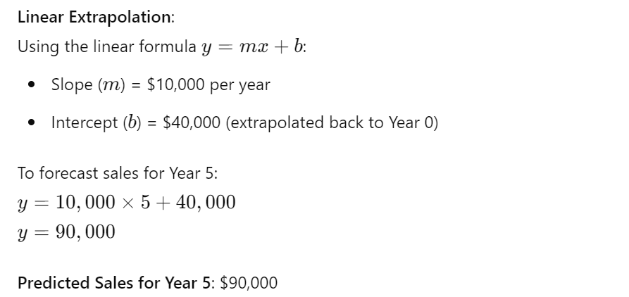
Script:A company wants to forecast its future sales based on historical data.

Historical data:

• Year 1: $50,000
• Year 2: $60,000
• Year 3: $70,000
• Year 4: $80,000

Sales have been increasing by $10,000 each year, indicating a linear trend.

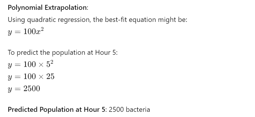
ScriptA biologist is studying the growth of a bacterial colony and observes that the growth rate is not linear but follows a quadratic trend.

Data:

• Hour 1: 100 bacteria
• Hour 2: 400 bacteria
• Hour 3: 900 bacteria
• Hour 4: 1600 bacteria

The relationship between time (x) and population (y) appears to follow a quadratic equation ( y = ax^2 + bx + c ).

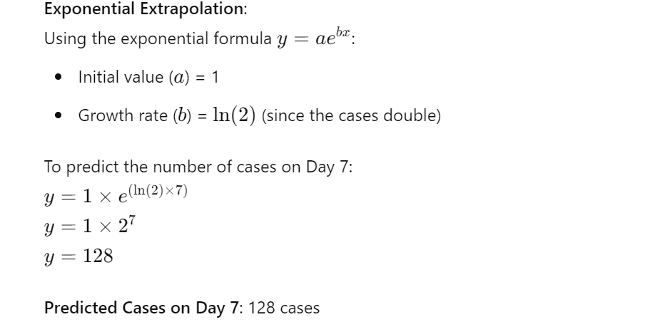
ScriptA researcher is tracking the spread of a viral infection and notices that the number of cases is doubling every day.

Data:

• Day 1: 1 case
• Day 2: 2 cases
• Day 3: 4 cases
• Day 4: 8 cases

These data suggest exponential growth.

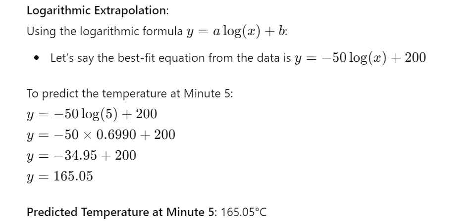
ScriptAn engineer studies the cooling rate of a heated object. The object cools rapidly at first and then more slowly, following a logarithmic trend.

Data:

• Minute 1: 150°C
• Minute 2: 100°C
• Minute 3: 75°C
• Minute 4: 60°C

Script:An analyst wants to smooth out daily fluctuations in stock prices to identify a long-term trend.

Data (last 5 days):

• Day 1: $150
• Day 2: $155
• Day 3: $160
• Day 4: $162
• Day 5: $165

Limitations and challenges

While extrapolation is a powerful tool, it carries significant risks:

• Uncertainty: The more you extrapolate your results, the greater the variability, that is, the less precise the results of the extrapolation will be.
• Assumptions: Although extrapolation has its disadvantage, it assumes that past trends will continue, but this may not be true most of the time.
• Overfitting: Using complicated models carries the risk that the model builds noise instead of the trend.
• Boundary conditions: Other things that are missing from extrapolation models are the limitations and barriers of physical and natural systems.

• Understanding the data: This means that once you have performed the extrapolation, you must perform a thorough analysis of the results obtained before the extrapolation to understand the trends and patterns in the data.
• Choose the right model: Choose the model with the format that works well with the nature of the data to be analyzed. It has been found that simpler models are better from a robustness standpoint.
• Validate the model: Given one part of the data, you need to check the output of the model and make corrections with the other part of the information.
• Consider external factors: In order not to compromise the validity of these findings, there are other factors and limitations regarding the study in question that must be taken into consideration:
• Quantifying uncertainty: Provides statistical probabilities along with extrapolated values ​​in order to have a wider range of possibilities.

Conclusion

Regression analysis is a fundamental statistical method necessary to estimate future values ​​as a continuation of presently observed values. Despite the obvious benefits of this approach in various fields, there are inherent risks and challenges that accompany it, as will be discussed later. This is so despite the fact that there are many types of regression analysis, each with its strengths and weaknesses, when the appropriate methods are applied, correct predictions can be achieved. To the same extent, extrapolation, if properly applied, remains a valuable aid to decision making and policy planning.

Frequently Asked Questions