Exploring Vanishing and Exploding Gradients in Neural Networks

Introduction

Deep learning is a fascinating field that explores the mysteries of gradients and their impact on neural networks. This journey delves into the depth of gradient descent, activation function anomalies, and weight initialization. Solutions like ReLU activation and gradient clipping promise to revolutionize deep learning, unlocking secrets for training success. Through vivid visualization and insightful analysis, we aim to forge a path towards neural networks that realize their full potential and redefine the future of ai. In this article we will understand vanishing and exploding gradients in neural networks in detail.

Learning Objectives

• Understand the concepts of vanishing and exploding gradients in deep learning.
• Learn methods to detect vanishing and exploding gradients during training.
• Explore strategies to mitigate vanishing and exploding gradients effectively.
• Gain insights into visualizing the effects of vanishing and exploding gradients in neural networks.
• Implement techniques such as proper weight initialization, ReLU activation, batch normalization, gradient clipping, and ResNet blocks to handle vanishing and exploding gradients in practice.

What is Gradient Descent?

Gradient descent is like the engine driving the optimization process in neural network training. It’s the method we use to tweak the inner workings of the network. However, sometimes it encounters problems. Picture this: the engine suddenly stalls or goes into overdrive. That’s what happens when gradients vanish or explode. When gradients vanish, the adjustments become too tiny, slowing down progress. Conversely, when they explode, adjustments become too big, throwing everything off course. Understanding how gradient descent interacts with these issues is crucial for ensuring smooth training and better performance from our neural networks.

If you’re seeking to expand your expertise in data analysis and visualization, consider enrolling in our BlackBelt program.

What are Vanishing Gradients?

Vanishing gradients occur when the neural network’s parameters become small during training, making it difficult for the network to learn from earlier layers. This results in slow or non-optimal performance. Detecting vanishing gradients involves monitoring their magnitude during training. Overcoming this issue involves careful initialization of network weights, activation functions to mitigate gradient attenuation, and techniques like skip connections for smoother gradient flow.

What are Exploding Gradients?

Exploding gradients occur when neural network parameters become too large during training, causing erratic and unstable behavior. Detecting these gradients involves monitoring their magnitude, especially for sudden spikes exceeding expected bounds. Techniques like gradient clipping and batch normalization help limit the magnitude of gradients and stabilize the training process, ensuring smoother gradient updates. Overcoming this issue is crucial for optimizing training algorithms.

Scenarios Where Vanishing and Exploding Gradient Occur

Let us now discuss where vanishing and exploding gradient can occur:

Occurrence of Vanishing Gradient

• The vanishing gradient problem occurs when the gradients in deep neural networks with more layers become smaller due to backpropagate, a common issue in deep feedforward and deep convolutional neural networks.
• Recurrent neural networks and LSTM networks struggle to learn long-term dependencies due to the repeated multiplication of small gradients, which can cause them to vanish over time steps.
• Saturating activation functions like sigmoid and tanh can lead to the vanishing gradient problem, as their gradients become small for large inputs, resulting in output values close to 0 or 1.

Occurrence of Exploding Gradient

• Recurrent neural networks with large weight initialization can cause gradients to exponentially grow during backpropagation, causing the exploding gradient problem.
• Large learning rates can lead to unstable updates and the exploding gradient problem when the gradients become extremely large.
• Unbounded activation functions in models like ReLU can lead to unbounded gradients, causing the exploding gradient problem when used without proper initialization or normalization techniques.
• Large input values or gradients can cause network propagation and explosion of gradients when used in training.

Major Causes of Vanishing Gradient 

Activation functions like sigmoid and hyperbolic tangent have saturating regions where gradients become small, leading to zero derivatives and vanishing gradients during backpropagation. This issue is more pronounced in deep networks due to multiple layers applying saturating activation functions. ReLU (Rectified Linear Unit) activation function addresses this issue by maintaining a constant positive gradient for positive inputs, preventing saturation and alleviating the vanishing gradient problem.

Poor weight initialization strategies can worsen the vanishing gradient problem by causing activations and gradients to shrink as they propagate through the network, resulting in vanishing gradients.

Xavier/Glorot initialization techniques aim to prevent exploding gradients by scaling initial weights based on the number of input and output units of each layer, thereby maintaining a reasonable range of activations and gradients.

Deep neural networks with multiple layers have long back-propagation paths, causing gradients to become smaller as they propagate backward. This issue is particularly prevalent in Recurrent Neural Networks (RNNs), as gradients can diminish exponentially over time due to repeated multiplication. Techniques like skip connections and gating mechanisms are used to improve gradient flow and mitigate the vanishing gradient problem in deep networks, such as residual networks and LSTMs and GRUs.

Major Causes of Exploding Gradient

Incorrect weight initialization in deep neural networks can cause exploding gradients during training. If weights are initialized with large values, subsequent updates during backpropagation can result in even larger gradients. For instance, weights from a normal distribution with a large standard deviation can cause exponential growth during training.

Large input values or gradients in a network can lead to exploding gradients, as activation functions may produce large output values, resulting in large gradients during backpropagation. Similarly, if the gradients themselves are very large, subsequent updates to the weights can further amplify the gradients, causing them to explode.

Poorly chosen activation functions, like the exponential function in ReLU activation, can cause gradient explosions for large positive inputs due to their derivative becoming large as input values increase. High learning rates can lead to unstable training and large gradients, as the optimization algorithm may overshoot the minimum of the loss function, causing the gradients to become large.

Methods to Mitigate Vanishing and Exploding Gradient

Let us now explore methods to mitigate vanishing and exploding gradient:

Weight Initialization

• Exploding Gradients: Large initial weights can lead to exploding gradients during backpropagation. Weight initialization techniques like Xavier (Glorot) and He initialization aim to keep the variance of activations and gradients approximately constant across layers. This helps in preventing gradients from becoming too large.
• Vanishing Gradients: Small initial weights can cause gradients to vanish as they propagate through layers. Proper initialization ensures that the gradients neither explode nor vanish.

Activation Functions

• ReLU and its Variants: ReLU, along with its variants like Leaky ReLU, Parametric ReLU, and Exponential ReLU, is a computationally efficient activation function used in deep learning models to mitigate vanishing gradients by avoiding saturation in the positive region.
• Sigmoid and Tanh: Sigmoid and tanh activations, while still used in some contexts, are less common in deeper networks due to their vanishing gradients and saturation at extreme values.

Batch Normalization

• Batch normalization (BN) normalizes the activations of each layer, which reduces the internal covariate shift. By stabilizing the distribution of inputs to each layer, BN helps in mitigating vanishing gradients and accelerating convergence during training.
• BN also acts as a regularizer, reducing the reliance on techniques like dropout and weight decay.

Gradient Clipping

• Gradient clipping is a technique used in recurrent neural networks (RNNs) to limit the size of gradients during backpropagation, preventing them from exploding and imposing a threshold to prevent excessive growth.

Residual Connections (ResNets)

• Residual connections introduce skip connections that allow gradients to flow more easily during training. By mitigating vanishing gradients, ResNets enable the training of very deep networks with hundreds or even thousands of layers.

Implementation of Gradients

We will create simple dense network with 10 hidden layers.

Step1: Importing Necessary Libraries

import numpy as np
import matplotlib.pyplot as plt
import tensorflow as tf
from tensorflow.keras.models import Sequential
from tensorflow.keras.datasets import mnist
from tensorflow.keras.layers import Dense, Activation, 
  BatchNormalization, Reshape, Conv2D, MaxPooling2D, Flatten
from tensorflow.keras.optimizers import Adam
from tensorflow.keras.callbacks import LearningRateScheduler
from tensorflow.keras.initializers import glorot_uniform
from tensorflow.keras.constraints import MaxNorm

Step2: Loading and Preprocessing of Dataset

# Generate dummy data (e.g., MNIST)
(X_train, y_train), _ = tf.keras.datasets.mnist.load_data()
X_train = X_train.reshape(-1, 28*28) / 255.0

num_classes = 10

Step3: Model Creation and Training

# Define a function to create a deep neural network with sigmoid activation
def create_deep_sigmoid_model():
    model = Sequential()
    model.add(Dense(256, input_dim=784, activation='sigmoid'))  # Input layer
    # Add multiple hidden layers with sigmoid activation
    for _ in range(10):
        model.add(Dense(256, activation='sigmoid'))
    model.add(Dense(10, activation='softmax'))  # Output layer
    return model

# Create and compile the model
model = create_deep_sigmoid_model()
model.compile(optimizer="adam", loss="sparse_categorical_crossentropy", 
            metrics=('accuracy'))

# Train the model
history = model.fit(X_train, y_train, epochs=10, batch_size=32, verbose=1)

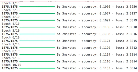
Here we can see that even though there is a decrease in the loss it is very less, after some epochs the loss reaches a plateau where there is no decrease in loss. This is a indication that there is vanishing gradient problem. 

Step4: Creating Visualization 

# Function to visualize the weights
def visualize_weights(model):
    all_weights = ()
    for layer in model.layers:
        if isinstance(layer, tf.keras.layers.Dense):
            weights = layer.get_weights()(0)
            all_weights.extend(weights.flatten())
    plt.hist(all_weights, bins=30)
    plt.title('Histogram of Weights')
    plt.xlabel('Weight Value')
    plt.ylabel('Frequency')
    plt.show()

# Visualize the weights of the model
visualize_weights(model)

In the above visualization we can see that the gradients are dense in range of gradient gradient value -0.1 to 0.1 this shows that there are high chances of vanishing gradients. 

# Plot the training history (accuracy)
plt.plot(history.history('accuracy'), label="accuracy")
plt.xlabel('Epoch')
plt.ylabel('Accuracy')
plt.title('Accuracy Convergence')
plt.legend()
plt.show()

In this image we can observe that after 3 epochs there is no visible increase in accuracy as the accuracy peaks at 11.2% and the model stops to learn. There is no convergence in accuracy happening, These is also indications of vanishing gradient. 

Using ReLU Throughout the Model

Now lets use the techniques that we discussed like Proper weight initialization, Using ReLU throughout the model instead of Sigmoid, Batch Normalization, ResNet Block.

Step1: Creating validation Data

Creating validation data as ResNet is a complex model and can get 100% accuracy when given enough epochs

# Generate dummy data (e.g., MNIST)
(X_train, y_train), _ = tf.keras.datasets.mnist.load_data()
X_train = X_train.reshape(-1, 28*28) / 255.0

num_classes = 10

Step2: Weight Initialization, Activation Function, Batch Normalization

# Weight Initialization (Glorot Uniform)
initializer = glorot_uniform()

# Activation Function (ReLU)
activation = 'relu'

# Batch Normalization
use_batch_norm = True

Step3: Model Creation

# Define ResNet Block Layer

class ResNetBlock(tf.keras.layers.Layer):
    def __init__(self, num_filters, kernel_size, strides=(1, 1), 
                  activation='relu', batch_norm=True):
        super(ResNetBlock, self).__init__()
        self.conv1 = Conv2D(num_filters, kernel_size, 
                    strides=strides, padding='same',kernel_initializer="he_normal")
        self.activation1 = Activation(activation)
        self.batch_norm1 = BatchNormalization() if batch_norm else None
        self.conv2 = Conv2D(num_filters, kernel_size,
                                 padding='same', kernel_initializer="he_normal")
          self.activation2 = Activation(activation)
        self.batch_norm2 = BatchNormalization() if batch_norm else None
        self.add_layer = Conv2D(num_filters, (1, 1), strides=strides, padding='same', 
                kernel_initializer="he_normal") if strides != (1, 1) else None
        self.activation3 = Activation(activation)

    def call(self, inputs, training=False):
        x = self.conv1(inputs)
        x = self.activation1(x)
        if self.batch_norm1:
            x = self.batch_norm1(x, training=training)
        x = self.conv2(x)
        x = self.activation2(x)
        if self.batch_norm2:
            x = self.batch_norm2(x, training=training)
        if self.add_layer:
            inputs = self.add_layer(inputs)
        x = tf.keras.layers.add((x, inputs))
        x = self.activation3(x)
        return x

# Define ResNet Model
def resnet_model():
    input_shape = (28, 28, 1)
    num_classes = 10
    model = Sequential()
    model.add(Conv2D(64, (7, 7), strides=(2, 2), padding='same', 
          input_shape=input_shape, kernel_initializer="he_normal"))
    model.add(Activation('relu'))
    model.add(BatchNormalization())
    model.add(MaxPooling2D((3, 3), strides=(2, 2), padding='same'))
    model.add(ResNetBlock(64, (3, 3), batch_norm=True))
    model.add(ResNetBlock(64, (3, 3), batch_norm=True))
    model.add(ResNetBlock(128, (3, 3), strides=(2, 2), batch_norm=True))
    model.add(ResNetBlock(128, (3, 3), batch_norm=True))
    model.add(ResNetBlock(256, (3, 3), strides=(2, 2), batch_norm=True))
    model.add(ResNetBlock(256, (3, 3), batch_norm=True))
    model.add(Flatten())
    model.add(Dense(num_classes, activation='softmax'))

    return model

Step4: Model Training

# Build the model

model = resnet_model()

# Compile the model
model.compile(optimizer="adam", loss="sparse_categorical_crossentropy", metrics=('accuracy'))

# Train the model
history = model.fit(X_train, y_train, epochs=10, batch_size=32, verbose=1)

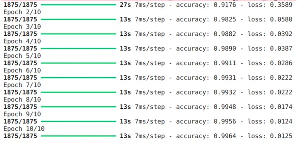
From the above image we can see that there is good decrease in loss and increase in accuracy. Hence we can say that we overcome the vanishing gradient problem. 

Step5: Visualization for Gradients and Accuracy

plt.plot(history.history('accuracy'), label="train_accuracy", marker="s", markersize=4)
plt.xlabel('Epoch')
plt.ylabel('Accuracy')
plt.ylim(0.90, 1)
plt.legend(loc="lower right")

Here we can see that the convergence of the accuracy is fast, hence proving us that there is very less vanishing gradient problem. 

# Function to visualize the weights

def visualize_weights(model):
    all_weights = ()
    for layer in model.layers:
        if isinstance(layer, tf.keras.layers.Dense):
            weights = layer.get_weights()(0)
            all_weights.extend(weights.flatten())
    plt.hist(all_weights, bins=30)
    plt.title('Histogram of Weights')
    plt.xlabel('Weight Value')
    plt.ylabel('Frequency')
    plt.show()

# Visualize the weights of the model
visualize_weights(model)

From the weight distribution we can see that weights are well distributed and does not have one dense region, hence we can say there is no or very less vanishing gradient problem.

Implementing Exploring Gradient

Now that we have seen how to mitigate vanishing gradient we will move on to Exploding Gradient

Step1: Creating a Linear Model

# Define a function to create a deep neural network with linear activation
def create_deep_linear_model(num_layers=20):
    model = Sequential()
    model.add(Dense(256, input_dim=784, activation='linear'))  # Input layer
    # Add multiple hidden layers with linear activation
    for _ in range(num_layers):
        model.add(Dense(256, activation='linear'))
    model.add(Dense(10, activation='softmax'))  # Output layer
    return model

Step2: Model Compilation and Declaration Gradient Norm Function 

# Create and compile the model
model = create_deep_linear_model()
model.compile(optimizer="adam", loss="sparse_categorical_crossentropy", 
               metrics=('accuracy'))

# Define a function to compute gradient norms for weights only
def compute_weight_gradient_norms(model, x, y):
    with tf.GradientTape() as tape:
        predictions = model(x)
        loss = tf.reduce_mean(tf.keras.losses.sparse_categorical_crossentropy(y, predictions))
    gradients = tape.gradient(loss, model.trainable_variables)
    weight_gradients = (grad for i, grad in enumerate(gradients) 
                        if 'bias' not in model.weights(i).name)
    weight_gradient_norms = (tf.norm(grad).numpy() for grad in weight_gradients)
    return weight_gradient_norms

Step3: Training Our Model 

# Train the model and compute gradient norms
history = {'accuracy': (), 'loss': (), 'gradient_norms': ()}

for epoch in range(10):
    # Train for one epoch
    model.fit(X_train, y_train, batch_size=32, verbose=0)
    # Evaluate accuracy and loss
    loss, accuracy = model.evaluate(X_train, y_train, verbose=0)
    history('accuracy').append(accuracy)
    history('loss').append(loss)
    # Compute gradient norms
    gradient_norms = compute_gradient_norms(model, X_train, y_train)
    history('gradient_norms').append(gradient_norms)

Step4: Visualization

# Plot the training history (accuracy and loss)
plt.figure(figsize=(12, 6))
plt.subplot(1, 2, 1)
plt.plot(history('accuracy'), label="accuracy")
plt.plot(history('loss'), label="loss")
plt.xlabel('Epoch')
plt.ylabel('Value')
plt.title('Training History')
plt.legend()

# Plot gradient norms
plt.subplot(1, 2, 2)
for i in range(len(history('gradient_norms')(0))):
    gradient_norms_epoch = (gradient_norms(i) for gradient_norms in history('gradient_norms'))
    plt.plot(gradient_norms_epoch, label=f'Layer {i+1}')
plt.xlabel('Epoch')
plt.ylabel('Gradient Norm')
plt.title('Gradient Norms')
plt.legend()
plt.tight_layout()
plt.show()

From the above visualization we can see that there is a exploding in gradient in 3rd epoch as the loss and gradient norm for weights has sky rocketed. It clearly shows that there is gradients exploding in our model which makes it unstable and not learn. 

Using Gradient Clipping

Now lets use techniques like gradient clipping.

Step1: Use of Model Architecture

# Define a function to create a deep neural network with linear activation
def create_deep_linear_model(num_layers=20):
    model = Sequential()
    model.add(Dense(256, input_dim=784, activation='linear'))  # Input layer
    # Add multiple hidden layers with linear activation
    for _ in range(num_layers):
        model.add(Dense(256, activation='linear'))
    model.add(Dense(10, activation='softmax'))  # Output layer
    return model

Step2: Using Compile with Clipping

We will be using the same compile but with clipping.

# Create and compile the model
model = create_deep_linear_model()
optimizer = tf.keras.optimizers.Adam(learning_rate=0.001, clipnorm=1.0)  # Gradient clipping
model.compile(optimizer=optimizer, loss="sparse_categorical_crossentropy", metrics=('accuracy'))

Step3: Function to Compute Gradient Norm for Weights

# Define a function to compute gradient norms for weights only
def compute_weight_gradient_norms(model, x, y):
    with tf.GradientTape() as tape:
        predictions = model(x)
        loss = tf.reduce_mean(tf.keras.losses.sparse_categorical_crossentropy(y, predictions))
    gradients = tape.gradient(loss, model.trainable_variables)
    weight_gradients = (grad for i, grad in enumerate(gradients) 
                        if 'bias' not in model.weights(i).name)
    weight_gradient_norms = (tf.norm(grad).numpy() for grad in weight_gradients)
    return weight_gradient_norms

Step4: Training the Model

# Train the model and compute gradient norms
history = {'accuracy': (), 'loss': (), 'weight_gradient_norms': ()}

for epoch in range(10):
    # Train for one epoch
    model.fit(X_train, y_train, batch_size=32, verbose=0)
    # Evaluate accuracy and loss
    loss, accuracy = model.evaluate(X_train, y_train, verbose=0)
    history('accuracy').append(accuracy)
    history('loss').append(loss)
    # Compute gradient norms for weights only
    weight_gradient_norms = compute_weight_gradient_norms(model, X_train, y_train)
    history('weight_gradient_norms').append(weight_gradient_norms)

Step5: Visualization

# Plot the training history (accuracy and loss)
plt.figure(figsize=(12, 6))
plt.subplot(1, 2, 1)
plt.plot(history('accuracy'), label="accuracy")
plt.plot(history('loss'), label="loss")
plt.xlabel('Epoch')
plt.ylabel('Value')
plt.title('Training History'
plt.legend()

# Plot gradient norms for weights only
plt.subplot(1, 2, 2)
for i in range(len(history('weight_gradient_norms')(0))):
    weight_gradient_norms_epoch = (gradient_norms(i) 
               for gradient_norms in history('weight_gradient_norms'))
    plt.plot(weight_gradient_norms_epoch, label=f'Layer {i+1}')

plt.xlabel('Epoch')
plt.ylabel('Gradient Norm (Weights)')
plt.title('Gradient Norms for Weights')
plt.legend()
plt.tight_layout()
plt.show()

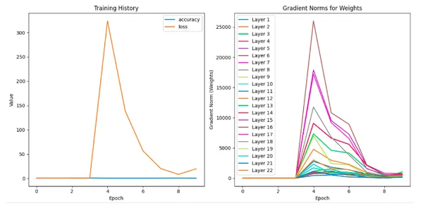
In the above plot we can see that the loss decreases gradually, training accuracy converges as the gradients are stable. Interpretation of these graphs are important as one may suggest that there is a spike in gradient norm. You can compare the magnitude of the graphs of model without clipping and infer that these are just gradual fluctuations. 

Conclusion

This article explores the visualization and mitigation of vanishing and exploding gradients in deep neural networks. It examines vanishing gradients in networks with sigmoid activation functions, highlighting causes like activation function saturation and weight initialization. Mitigation strategies include ReLU activation and proper weight initialization, which stabilize training dynamics. The article then addresses exploding gradients in networks with linear activations, implementing gradient clipping as a mitigation technique. This method stabilizes training and ensures convergence, emphasizing the importance of understanding and addressing gradient challenges for successful deep learning model training.

If you’re seeking to expand your expertise in data analysis and visualization, consider enrolling in our BlackBelt program.

Frequently Asked Questions