Chronos-Bolt is the newest addition to AutoGluon-TimeSeries, delivering accurate zero-shot forecasting up to 250 times faster than the original Chronos models (1).
Time series forecasting plays a vital role in guiding key business decisions across industries such as retail, energy, finance, and healthcare. Traditionally, forecasting has relied on statistical models (2) like ETS and ARIMA, which remain strong baselines, particularly when training data is limited. Over the past decade, advancements in deep learning have spurred a shift toward so-called global models such as DeepAR (3) and PatchTST (4). These approaches train a single deep learning model across multiple time series in a dataset—for example, sales across a broad e-commerce catalog or observability metrics for thousands of customers.
Foundation models (FMs) such as <a target="_blank" href="https://www.amazon.science/blog/adapting-language-model-architectures-for-time-series-forecasting” target=”_blank” rel=”noopener”>Chronos (1) have taken the idea of training a single model across multiple time series a significant step further. These models are pretrained on a vast corpus of real and synthetic time series data, covering diverse domains, frequencies, and history lengths. As a result, they enable zero-shot forecasting—delivering accurate predictions on unseen time series datasets. This lowers the entry barrier to forecasting and greatly simplifies forecasting pipelines by providing accurate forecasts without the need for training. Chronos models have been downloaded over 120 million times from <a target="_blank" href="https://huggingface.co/collections/amazon/chronos-models-and-datasets-65f1791d630a8d57cb718444″ target=”_blank” rel=”noopener”>Hugging Face and are available for amazon SageMaker customers through AutoGluon-TimeSeries and amazon SageMaker JumpStart.
In this post, we introduce Chronos-Bolt, our latest FM for forecasting that has been integrated into AutoGluon-TimeSeries.
Introducing Chronos-Bolt
Chronos-Bolt is based on the T5 encoder-decoder architecture (5) and has been trained on nearly 100 billion time series observations. It chunks the historical time series context into patches of multiple observations, which are then input into the encoder. The decoder then uses these representations to directly generate quantile forecasts across multiple future steps—a method known as direct multi-step forecasting. This differs from the original Chronos models that rely on autoregressive decoding. The chunking of time series and direct multi-step forecasting makes Chronos-Bolt up to 250 times faster and 20 times more memory-efficient than the original Chronos models.
The following plot compares the inference time of Chronos-Bolt against the original Chronos models for forecasting 1024 time series with a context length of 512 observations and a prediction horizon of 64 steps.
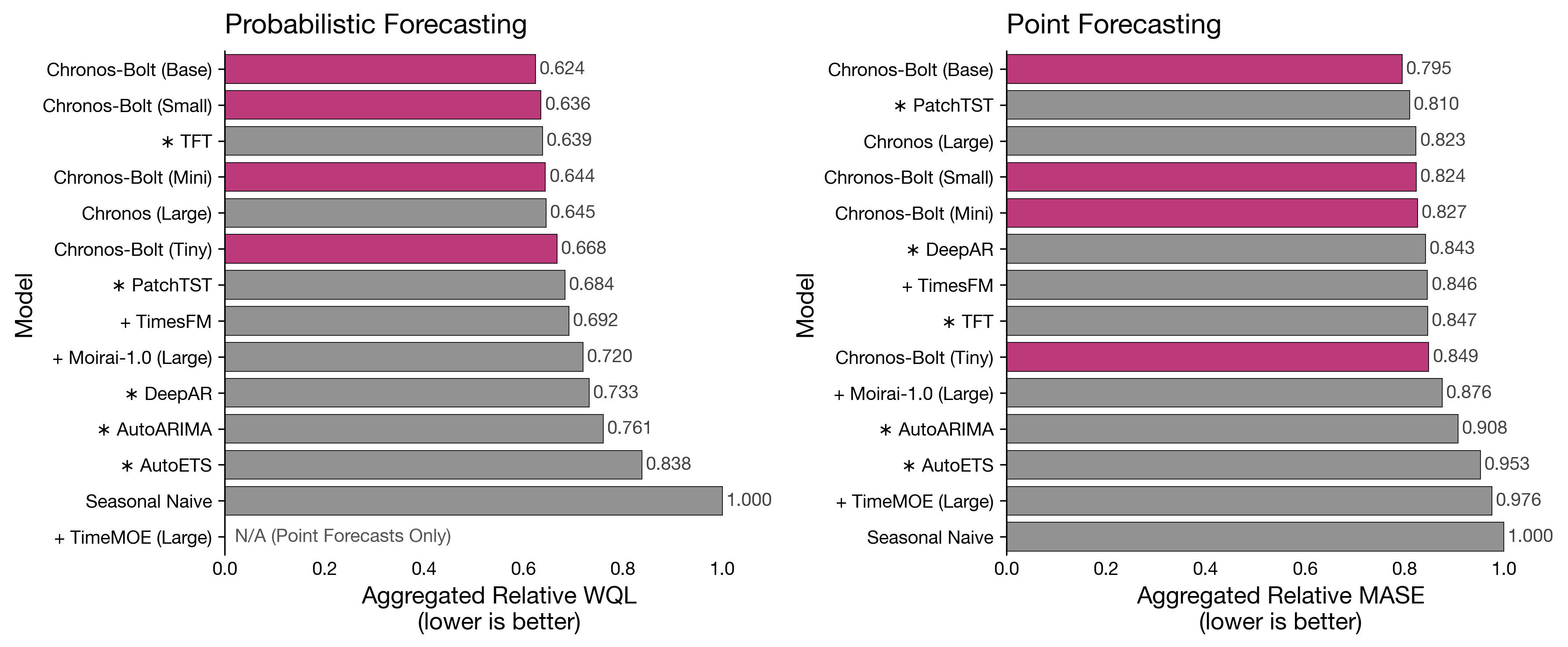
Chronos-Bolt models are not only significantly faster, but also more accurate than the original Chronos models. The following plot reports the probabilistic and point forecasting performance of Chronos-Bolt in terms of the <a target="_blank" href="https://auto.gluon.ai/stable/tutorials/timeseries/forecasting-metrics.html#autogluon.timeseries.metrics.WQL” target=”_blank” rel=”noopener”>Weighted Quantile Loss (WQL) and the <a target="_blank" href="https://auto.gluon.ai/stable/tutorials/timeseries/forecasting-metrics.html#autogluon.timeseries.metrics.MASE” target=”_blank” rel=”noopener”>Mean Absolute Scaled Error (MASE), respectively, aggregated over 27 datasets (see (1) for dataset details). Remarkably, despite having no prior exposure to these datasets during training, the zero-shot Chronos-Bolt models outperform commonly used statistical models and deep learning models that have been trained on these datasets (highlighted by *). Furthermore, they also perform better than other FMs, denoted by a +, which indicates that these models were pretrained on certain datasets in our benchmark and are not entirely zero-shot. Notably, Chronos-Bolt (Base) also surpasses the original Chronos (Large) model in terms of the forecasting accuracy while being over 600 times faster.

Chronos-Bolt models are now available on <a target="_blank" href="https://huggingface.co/collections/amazon/chronos-models-and-datasets-65f1791d630a8d57cb718444″ target=”_blank” rel=”noopener”>Hugging Face in four sizes—Tiny (9M), Mini (21M), Small (48M), and Base (205M)—and can also be used on the CPU.
Solution overview
In this post, we showcase how to use Chronos-Bolt models using the familiar interface of AutoGluon-TimeSeries. AutoGluon-TimeSeries enables SageMaker customers to build and deploy models for time series forecasting, including FMs such as Chronos-Bolt and other global models, and effortlessly ensemble them with statistical models to maximize accuracy.
Perform zero-shot forecasting with Chronos-Bolt
To get started, you need to install AutoGluon v1.2 by running the following command in an amazon SageMaker Studio notebook or in the terminal:
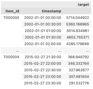
AutoGluon-TimeSeries uses the TimeSeriesDataFrame to work with time series datasets. The TimeSeriesDataFrame expects data in the long dataframe format with at least three columns: an ID column denoting the IDs of individual time series in the dataset, a timestamp column, and a target column that contains the raw time series values. The timestamps must be uniformly spaced, with missing observations denoted by NaN and Chronos-Bolt will handle them appropriately. The following snippet loads the Australian Electricity dataset (6) that contains electricity demand data at 30-minute intervals for five Australian states into a TimeSeriesDataFrame:

The next step involves fitting a TimeSeriesPredictor on this data:
We have specified that the TimeSeriesPredictor should produce forecasts for the next 48 steps, or 1 day in this case. AutoGluon-TimeSeries offers various presets that can be used when fitting the predictor. The bolt_base preset, used in this example, employs the Base (205M) variant of Chronos-Bolt for zero-shot inference. Because no model fitting is required for zero-shot inference, the call to fit() returns almost instantaneously. The predictor is now ready to generate zero-shot forecasts, which can be done through the predict method:
AutoGluon-TimeSeries generates both point and probabilistic (quantile) forecasts for the target value. The probabilistic forecast captures the uncertainty of the target value, which is essential for many planning tasks.

We can also visualize the predictions and compare them against the ground truth target value over the forecast horizon:
Chronos-Bolt generates an accurate zero-shot forecast, as shown in the following plot illustrating point forecasts and the 80% prediction intervals.

Fine-tune Chronos-Bolt with AutoGluon
So far, we have used Chronos-Bolt in inference-only mode for zero-shot forecasting. However, AutoGluon-TimeSeries also allows you to fine-tune Chronos-Bolt on your specific datasets. We recommend using a GPU instance such as g5.2xlarge for fine-tuning. The following snippet specifies two settings for the Chronos-Bolt (Small, 48M) model: zero-shot and fine-tuned. AutoGluon-TimeSeries will perform a lightweight fine-tuning of the pretrained model on the provided training data. We add name suffixes to identify the zero-shot and fine-tuned versions of the model.
The predictor will be fitted for at most 10 minutes, as specified by the time_limit. After fitting, we can evaluate the two model variants on the test data and generate a leaderboard:

Fine-tuning resulted in a significantly improved forecast accuracy, as shown by the test MASE scores. All AutoGluon-TimeSeries models report scores in a “higher is better” format, meaning that most forecasting error metrics like MASE are multiplied by -1 when reported.
Augment Chronos-Bolt with exogenous information
Chronos-Bolt is a univariate model, meaning it relies solely on the historical data of the target time series for making predictions. However, in real-world scenarios, additional exogenous information related to the target series (such as holidays or promotions) is often available. Using this information when making predictions can improve forecast accuracy. AutoGluon-TimeSeries now features covariate regressors, which can be combined with univariate models like Chronos-Bolt to incorporate exogenous information. A covariate regressor in AutoGluon-TimeSeries is a tabular regression model that is fit on the known covariates and static features to predict the target column at each time step. The predictions of the covariate regressor are subtracted from the target column, and the univariate model then forecasts the residuals.
We use a grocery sales dataset to demonstrate how Chronos-Bolt can be combined with a covariate regressor. This dataset includes three known covariates: scaled_price, promotion_email, and promotion_homepage, and the task is to forecast the unit_sales:

The following code fits a TimeSeriesPredictor to forecast unit_sales for the next 7 weeks. We have specified the target column we are interested in forecasting and the names of known covariates while constructing the TimeSeriesPredictor. Two configurations are defined for Chronos-Bolt: a zero-shot setting, which uses only the historical context of unit_sales without considering the known covariates, and a covariate regressor setting, which employs a CatBoost model as the covariate_regressor. We also use the target_scaler, which makes sure the time series have a comparable scale before training, which typically results in better accuracy.
After the predictor has been fit, we can evaluate it on the test dataset and generate the leaderboard. Using the covariate regressor with Chronos-Bolt improves over its univariate zero-shot performance considerably.

The covariates might not always be useful—for some datasets, the zero-shot model might achieve better accuracy. Therefore, it’s important to try multiple models and select the one that achieves the best accuracy on held-out data.
Conclusion
Chronos-Bolt models empower practitioners to generate high-quality forecasts rapidly in a zero-shot manner. AutoGluon-TimeSeries enhances this capability by enabling users to fine-tune Chronos-Bolt models effortlessly, integrate them with covariate regressors, and ensemble them with a diverse range of forecasting models. For advanced users, it provides a comprehensive set of features to customize forecasting models beyond what was demonstrated in this post. AutoGluon predictors can be seamlessly deployed to SageMaker using <a target="_blank" href="https://auto.gluon.ai/cloud/dev/index.html” target=”_blank” rel=”noopener”>AutoGluon-Cloud and the official Deep Learning Containers.
To learn more about using AutoGluon-TimeSeries to build accurate and robust forecasting models, explore our <a target="_blank" href="https://auto.gluon.ai/stable/tutorials/timeseries/index.html” target=”_blank” rel=”noopener”>tutorials. Stay updated by following AutoGluon on <a target="_blank" href="https://twitter.com/autogluon” target=”_blank” rel=”noopener”>x (formerly twitter) and starring us on GitHub!
References
(1) Ansari, Abdul Fatir, Lorenzo Stella, Ali Caner Turkmen, Xiyuan Zhang, Pedro Mercado, Huibin Shen, Oleksandr Shchur, et al. “Chronos: Learning the language of time series.” Transactions on Machine Learning Research (2024).
(2) Hyndman, R. J., and G. Athanasopoulos. “Forecasting: principles and practice 3rd Ed.” O Texts (2018).
(3) Salinas, David, Valentin Flunkert, Jan Gasthaus, and Tim Januschowski. “DeepAR: Probabilistic forecasting with autoregressive recurrent networks.” International Journal of Forecasting 36, no. 3 (2020): 1181-1191.
(4) Nie, Yuqi, Nam H. Nguyen, Phanwadee Sinthong, and Jayant Kalagnanam. “A time series is worth 64 words: long-term forecasting with transformers.” In The Eleventh International Conference on Learning Representations (2023).
(5) Raffel, Colin, Noam Shazeer, Adam Roberts, Katherine Lee, Sharan Narang, Michael Matena, Yanqi Zhou, Wei Li, and Peter J. Liu. “Exploring the limits of transfer learning with a unified text-to-text transformer.” Journal of Machine Learning Research 21, no. 140 (2020): 1-67.
(6) Godahewa, Rakshitha, Christoph Bergmeir, Geoffrey I. Webb, Rob J. Hyndman, and Pablo Montero-Manso. “Monash time series forecasting archive.” In NeurIPS Track on Datasets and Benchmarks (2021).
About the Authors
 Abdul Fatir Ansari is a Senior Applied Scientist at amazon Web Services, specializing in machine learning and forecasting, with a focus on foundation models for structured data, such as time series. He received his PhD from the National University of Singapore, where his research centered on deep generative models for images and time series.
 Caner Turkmen is a Senior Applied Scientist at amazon Web Services, where he works on research problems at the intersection of machine learning and forecasting. Before joining AWS, he worked in the management consulting industry as a data scientist, serving the financial services and telecommunications sectors. He holds a PhD in Computer Engineering from Bogazici University in Istanbul.
 Oleksandr Shchur is a Senior Applied Scientist at amazon Web Services, where he works on time series forecasting in AutoGluon. Before joining AWS, he completed a PhD in Machine Learning at the Technical University of Munich, Germany, doing research on probabilistic models for event data. His research interests include machine learning for temporal data and generative modeling.
 Lorenzo Stella is a Senior Applied Scientist at amazon Web Services, working on machine learning, forecasting, and generative ai for analytics and decision-making. He holds a PhD in Computer Science and Electrical Engineering from IMTLucca (Italy) and KU Leuven (Belgium), where his research focused on numerical optimization algorithms for machine learning and optimal control applications.
<script async src="//platform.twitter.com/widgets.js” charset=”utf-8″>


